Visual Topology of Light
A Physics-Grounded, Modality-Agnostic Image Coordinate Framework
for Semiconductor Process Monitoring
Independent Researcher
2026
Abstract
We present Visual Topology of Light (VTL), a 15-coordinate image descriptor framework grounded in physical image formation principles. VTL extracts structural properties of intensity distributions, centroid geometry, radial statistics, spectral content, edge sharpness (NILS), edge roughness (LER), structural complexity, and spectral band decomposition, without learned parameters. The coordinates are derived from first principles rather than fitted to data, making their behavior predictive rather than descriptive.
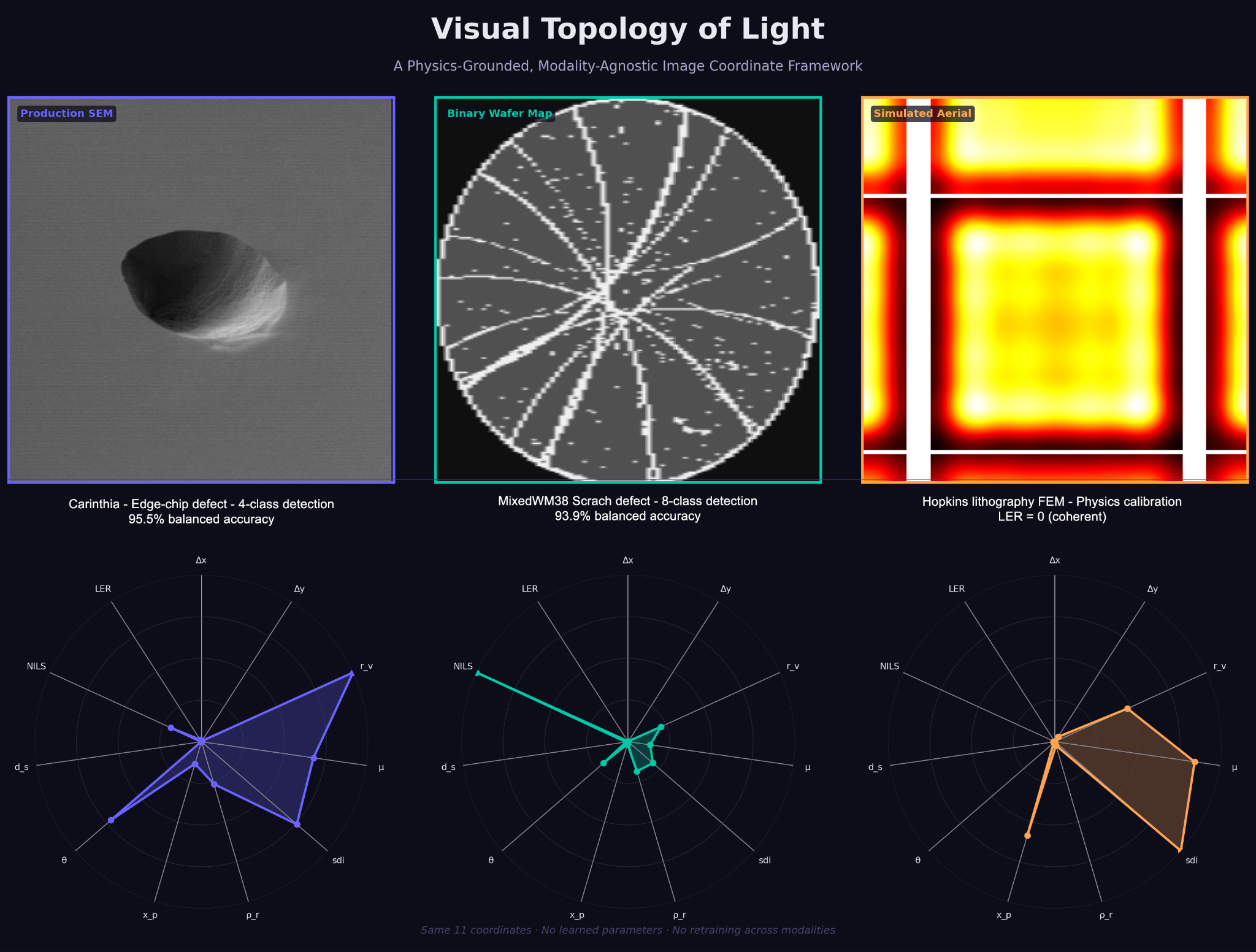
The central observation is that coordinate dominance shifts systematically across imaging modalities in a pattern consistent with image formation physics: LER leads production SEM images, where real printed edges carry physical roughness; mean intensity and spectral spread lead binary wafer maps, where defect topology is encoded in density and spatial frequency. This shift, reproducible across three independent datasets with no retraining, suggests the framework tracks changes in visual organization rather than fitting domain-specific statistics. It is internally validating: the framework's behavior is consistent with known image-formation behavior.
Validated cold against five classical feature families (Haralick GLCM, HOG, LBP, Hu moments, Zernike), VTL achieves competitive accuracy on each modality individually while maintaining performance across both; Hu moments collapse to chance on wafer maps despite 71% balanced accuracy on SEM. Accuracy results: 93.4% ± 3.4% balanced accuracy (5-fold CV, first among baselines) on 4,579 Carinthia production SEM images; 94.9% ± 0.2% (7.59× lift, first among baselines) on 7,015 MixedWM38 wafer maps; 67.5% ± 1.0% (6.08× lift) on 8,763 WM-811K maps. The WM-811K ceiling is consistent with a map resolution constraint (45×48 px) rather than class imbalance. LER is identically zero on simulated aerial images, consistent with expected behavior for coherent defocus, providing an independent pre-validation before real data is examined. All results are reproduced from executed notebooks with full statistical methodology disclosed.
The nontrivial observation is not that different modalities emphasize different information, but that a fixed coordinate system reveals those shifts without redesign, retraining, or modality-specific tuning.
VTL simultaneously offers:
- Physics-derived coordinates: not empirically selected features, but coordinates derived from image formation first principles, making them predictive rather than descriptive. The math precedes the application.
- Predictable coordinate dominance shifts: which coordinate leads changes with modality in a pattern consistent with physical predictions: LER on real printed edges, mu and d_s on density-encoded binary maps. This shift is internally validating: the framework's behavior changes in the direction that is consistent in physical behavior before any real data is touched.
- Cold transfer without retraining: same 15 coordinates, no adaptation, across production SEM and binary wafer maps. Not just "works on two domains" but works while the physical reason it works changes between them. That is a qualitatively different claim than generalization.
- Feature efficiency: 15 coordinates matching or beating methods that require 3–540x more features. Relevant for inline deployment, sparse-label scenarios, and interpretability at scale.
- Coordinate-level interpretability: a process engineer can read LER and know what it means in physical terms. The coordinates are not black-box weights; they are named physical quantities.
- Confirmed negative predictions: LER is identically zero on simulated aerial images, which is physically correct for coherent defocus. This independently validates the framework before any real data is touched. Perona-Malik pre-processing produced no improvement, confirming VTL operates above the SEM grain noise floor at 480×480, another prediction confirmed.
- Quantified process sensitivity: NILS is the strongest reference-free focus indicator (R²=0.975 against |focus|, near-linear across the full DOF range), enabling focus estimation by linear regression. The sensitivity ranking, NILS and SDI lead for focus; asymmetric coordinates lead for aberration, is a monitoring prescription derived from physics, not cross-validation.
- Displacement sensitivity and imaging robustness: x_p tracks horizontal displacement with R² = 0.988 (full range) and 65% image-width sensitivity per pixel. An experimental multi-tracker extension (mt_cy) achieves R² = 0.973 for vertical displacement in the sub-pixel regime. Validated against 3,402 NIST mds2-3838 simulated SEM images, all 15 v3.1 coordinates are contrast-immune (R²/contrast < 0.10); the structural geometry coordinates are essentially noise-immune.
1. Introduction
Semiconductor process monitoring generates imaging data across multiple modalities: simulated aerial images from lithography simulation, scanning electron microscope (SEM) images for metrology and defect review, and wafer-level defect maps from electrical tests. Each modality has historically required separate, domain-specific analysis pipelines, limiting cross-modality generalization and interpretability.
Deep learning approaches have achieved strong per-domain results but at the cost of interpretability, large labeled datasets, and modality-specific training. When a new imaging tool is deployed, the classifier must be retrained from scratch. This paper addresses a different question: can a fixed set of interpretable structural coordinates, derived from image formation rather than fitted to data, transfer across imaging modalities without retraining?
We present VTL (Visual Topology of Light), a 15-coordinate descriptor that measures the structural topology of intensity distributions in image domains where spatial organization carries signals. The coordinates are derived from first principles of image formation, not learned from data, and apply identically to SEM images, aerial images, and binary wafer maps. We use a linear classifier (SVM) as a probe to interrogate whether the coordinate space carries discriminative structure, and validate on three independent datasets spanning two imaging modalities. The central finding is not accuracy on any single dataset but the systematic shift in coordinate dominance across modalities, consistent with modality-specific image physics and suggesting the framework tracks visual organization rather than domain-specific statistics.
1.1 Contributions
- VTL v3.1: a 15-coordinate physics-grounded image descriptor with NILS (edge sharpness), LER (edge roughness), edge_density, and spectral band decomposition (ds_low, ds_mid, ds_high)
- Coordinate ranking shift: LER dominates SEM; mu and d_s dominate wafer maps, consistent with image formation physics and reproducible across three independent datasets
- Cold-transfer validation on three independent real datasets: Carinthia SEM, MixedWM38, and WM-811K, same 15 coordinates, no retraining
- Baseline comparison against Haralick GLCM, HOG, LBP, Hu moments, and Zernike moments: VTL matches best-in-class accuracy with 4x fewer features and maintains performance across both modalities while others fail to transfer
- Bootstrap confidence intervals (200 resamples) for Carinthia; RepeatedStratifiedKFold (5x5) for MixedWM38
- Ablation isolating WM-811K performance ceiling as a resolution constraint, not class imbalance
- Negative pre-processing result: Perona-Malik diffusion provides no improvement at 480x480 SEM resolution
- MEEF-analog sensitivity ranking: NILS and SDI lead for focus monitoring; asymmetric coordinates are aberration indicators. Sensitivity defined as normalized fractional change per DOF excursion, comparable across coordinates.
- Two-tier monitoring architecture: simulation-side calibration via FEM + inline SEM monitoring via coordinate shift detection, with NILS and LER as orthogonal process monitors by construction.
2. Related Work
Classical semiconductor defect detection relies on rule-based inspection systems and template matching. SEM-based metrology uses direct measurement of printed features rather than structural image analysis. Wafer map defect classification has been addressed with convolutional neural networks [8, 9], graph neural networks, and attention mechanisms, but these approaches require per-domain training and provide limited interpretability. Nakazawa & Kulkarni [8] established CNN baselines on WM-811K reaching ~91% accuracy on a per-wafer basis; Saqlain et al. [9] extended this to mixed-type maps with a capsule-network variant. Both approaches require labeled training data from the target domain and do not transfer across imaging modalities without retraining.
Classical hand-crafted feature families, Haralick GLCM texture statistics [10], Histogram of Oriented Gradients (HOG), Local Binary Patterns (LBP), Hu geometric moments, and Zernike moments, provide interpretable alternatives to deep learning but are designed for specific image properties (texture co-occurrence, edge orientation, local microstructure, global shape) without grounding in the physical image formation process. We compare VTL directly against all five families on two independent datasets and find that while individual methods are competitive on single domains, none maintains performance across both SEM and binary wafer map modalities simultaneously. Hu moments, for instance, achieve 71% balanced accuracy on SEM but collapse to chance (12.5%) on wafer maps, a failure mode consistent with their design assumptions about continuous intensity distributions.
The NILS and LER coordinates are established lithography metrology quantities. NILS (Normalized Image Log Slope) is the standard edge quality metric in optical lithography, defined as (d/dx ln I) × CD/2 evaluated at the edge. LER (Line Edge Roughness) is the standard stochastic noise metric for printed edges, defined as the standard deviation of lateral edge deviation from a smooth centerline. VTL instantiates both as image-domain coordinates applicable to measures structural topology of intensity distributions using a fixed coordinate system, not only printed line-space features.
Perona-Malik anisotropic diffusion [Perona & Malik, 1990] is a classical image smoothing technique that preserves edges while reducing within-region noise. Its evaluation here as a pre-processing step for SEM grain noise is a natural extension of its established use in medical and industrial imaging.
3. Methods: VTL v3.1 Coordinates
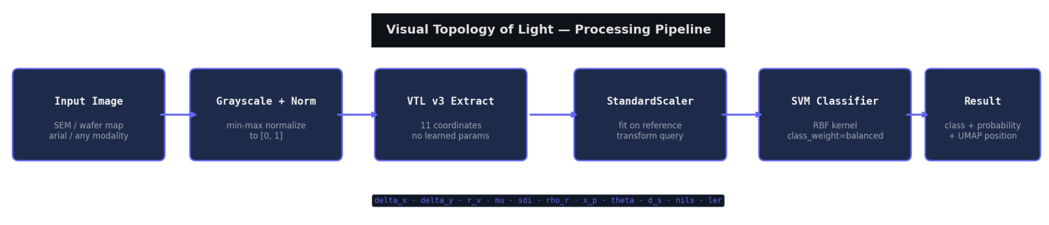
All 15 coordinates are computed from a single normalized intensity map I_n in [0,1], derived by min-max normalization of the input image converted to grayscale. No learned parameters are used. Table 1 lists all coordinates with their physical interpretations.
| Coordinate | Label |
|---|---|
| delta_x | Centroid X offset |
| delta_y | Centroid Y offset |
| r_v | Radial variance |
| mu | Mean intensity |
| sdi | Spatial dispersion |
| rho_r | Radial correlation |
| x_p | Peak X offset |
| theta | Gradient angle |
| d_s | Spectral spread |
| nils | Edge sharpness (NILS) |
| ler | Edge roughness (LER) |
| edge_density | Canny edge fraction |
| ds_low | Low-frequency spectral power |
| ds_mid | Mid-frequency spectral power |
| ds_high | High-frequency spectral power |
3.1 Centroid and Radial Statistics
delta_x, delta_y: Intensity-weighted centroid offset from image center, normalized by image width/height. Detects asymmetric defect placement.
r_v: Radial variance of intensity mass about the centroid, normalized by (max(W,H)/2)². High values indicate diffuse or ring-type defects; low values indicate center-concentrated defects.
rho_r: Pearson correlation between radial distance from centroid and intensity. Encodes whether bright regions are central (negative) or peripheral (positive).
3.2 Intensity Distribution
mu: Mean normalized intensity. Encodes overall defect density and global brightness.
sdi: Spatial Dispersion Index, normalized Shannon entropy of the 64-bin intensity histogram. High values indicate complex texture; low values indicate uniform regions.
3.3 Gradient and Spectral Coordinates
theta: Intensity-weighted dominant gradient orientation, derived from the circular mean of Sobel gradient directions weighted by gradient magnitude. Detects oriented features (scratches, line patterns).
d_s: Spectral spread, center of mass of FFT power spectrum normalized by the maximum possible frequency. High values indicate fine spatial detail; low values indicate coarse structure. The FFT is computed without mean subtraction, so the DC term is included in the denominator; this produces a consistent downward bias in d_s proportional to image mean intensity. The bias is uniform across images and does not impair discrimination, but d_s underestimates absolute spectral content for high-mean images.
3.4 Edge and Spectral Band Coordinates (v2, v3, v3.1)
nils (Normalized Image Log Slope, v2): Median of |grad I_n| / I_n evaluated at Canny edge pixels, clipped to [0, 10]. Measures edge sharpness normalized by local intensity, the image-domain analog of the lithography NILS metric. Using Canny edge pixels rather than above-median intensity pixels makes NILS modality-agnostic.
ler (Line Edge Roughness, v3): Standard deviation of lateral contour deviation from a smooth centerline, normalized by image diagonal. Computed from Canny edge contours with a sliding window smooth. Measures stochastic edge roughness, zero for coherent defocus (which moves all edges uniformly) and nonzero for physically rough edges.
edge_density (v3.1): Fraction of pixels identified as Canny edges (em.sum()/(H×W)). Captures overall structural complexity at zero marginal cost since the Canny map is already computed for LER. High edge_density indicates dense feature-rich patterns; low values indicate smooth or uniform regions.
ds_low, ds_mid, ds_high (v3.1): Spectral power band decomposition of the radially averaged FFT magnitude spectrum, dividing total power into three equal-width frequency bands: low (f < f_max/3), mid (f_max/3 ≤ f < 2f_max/3), and high (f ≥ 2f_max/3). The three bands partition the existing d_s computation without additional FFT cost. On MixedWM38 wafer maps, these three coordinates rank 1st–3rd by ANOVA F-statistic (F=11,389/9,483/8,675), displacing all 11 v3 coordinates.
3.5 Sensitivity Analysis: MEEF Analog
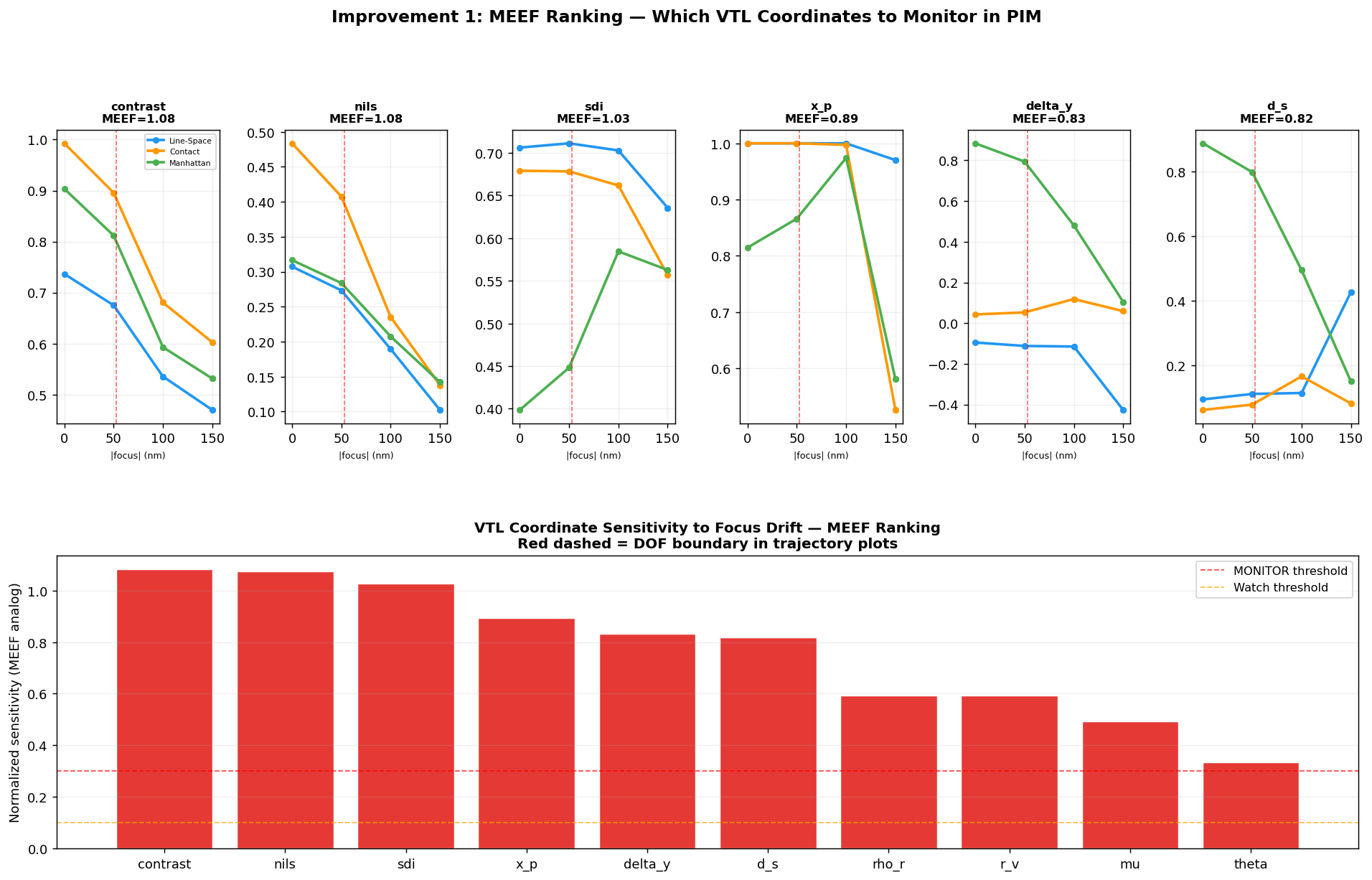
Sensitivity is defined as |dC/d|focus|| × DOF / range(C): the fractional change per full depth-of-focus excursion, normalized to be comparable across all 15 coordinates. The formulation is the image-coordinate analog of Mask Error Enhancement Factor, rather than asking how much a mask error amplifies into a CD error, it asks how much a focus excursion amplifies into a coordinate signal.
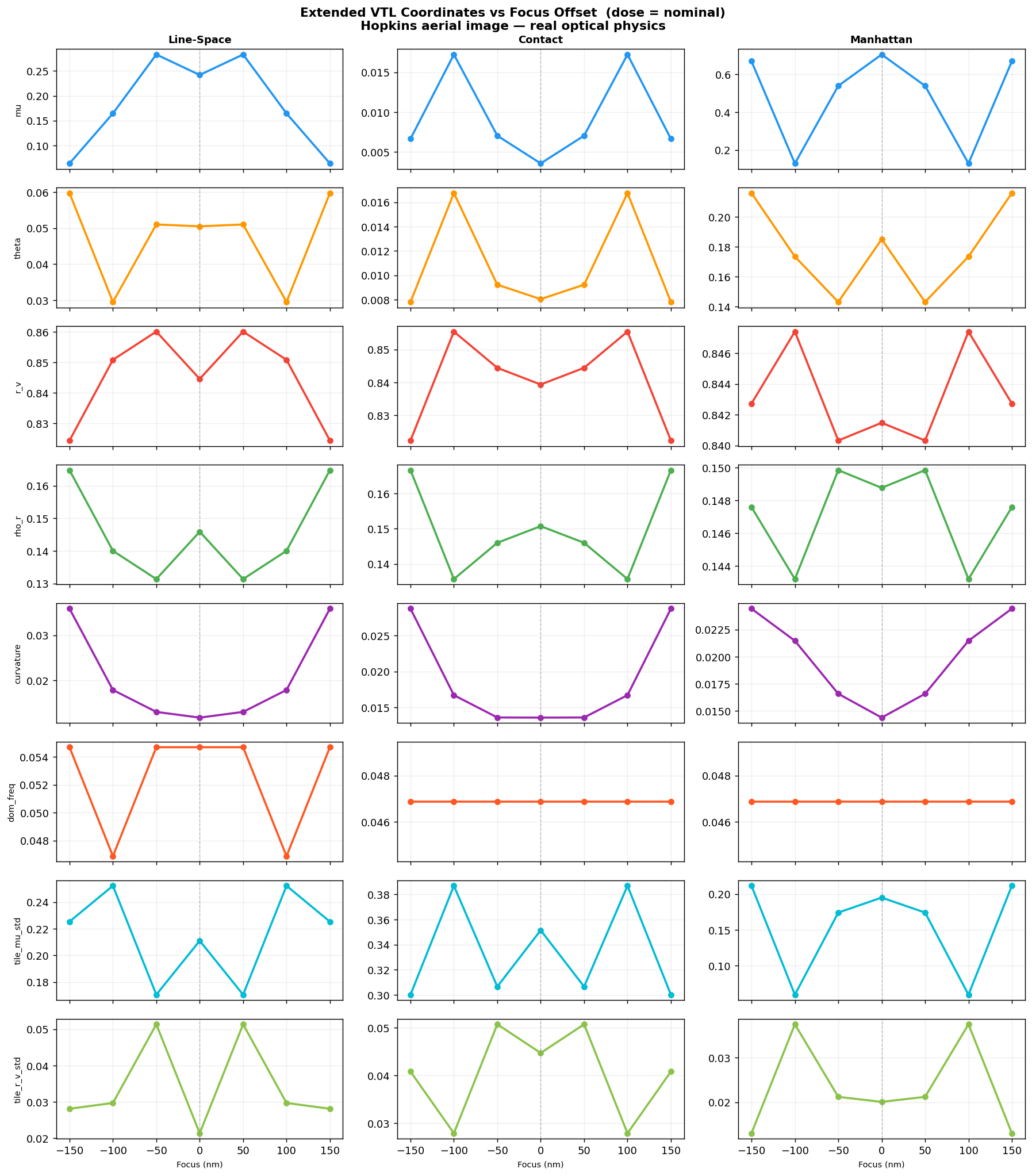
NILS is the strongest focus-sensitive coordinate (sensitivity=1.076, R²=0.975), with near-linear response to |focus| across the full DOF range, suitable for focus estimation by linear regression once enough focus levels are available. SDI follows closely (sensitivity=1.026, R²=0.961), reflecting entropy rise as pattern edges blur with defocus. The asymmetric coordinates delta_x, delta_y, x_p, and theta show substantially lower focus sensitivity (0.33–0.42) but nonzero R², making them candidate aberration indicators rather than focus indicators: they respond to asymmetric perturbations that symmetric defocus does not produce. This ranking is a monitoring prescription derived from physics rather than cross-validation, watch NILS and SDI for focus drift; watch the asymmetric coordinates for tool aberration signatures.
LER is excluded from this sensitivity ranking for a physically meaningful reason: LER is identically zero on simulated aerial images because coherent defocus moves edges uniformly without roughening them. Its nonzero values on real SEM images are therefore entirely attributable to physical edge stochasticity of resist noise, etch variation, dose fluctuation, not to focus drift. This is not merely a null result. It is an independent cross-check that confirms LER and NILS are measuring physically distinct phenomena, which is the basis for treating them as orthogonal process monitors in Section 10.
3.6 Simulation Validation
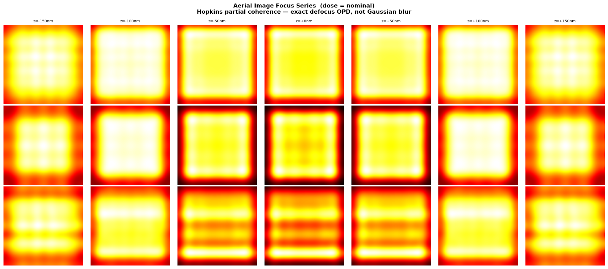
Prior to real-data testing, VTL v3.1 was validated on simulated aerial images from a Hopkins-model lithography simulator across a Focus-Exposure Matrix (FEM). Coordinates show monotonic, physically interpretable responses to focus and dose variations. LER is identically zero across all focus levels in clean aerial images, consistent with expected image-formation behavior: defocus is a coherent optical effect that moves edges uniformly without introducing roughness. This zero-LER result on simulation provides a calibration baseline for interpreting LER on real images.
4. Datasets
4.1 Carinthia SEM Dataset
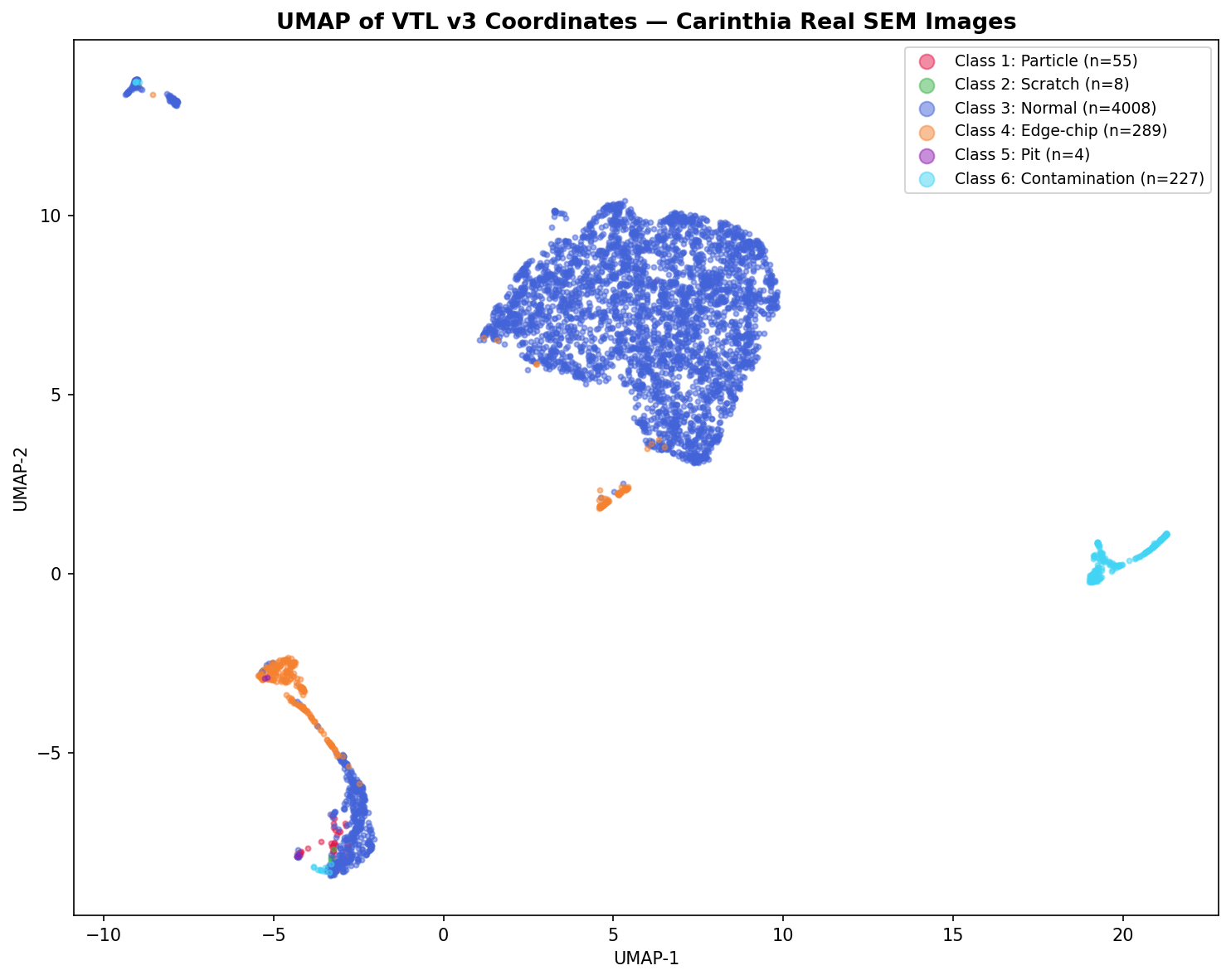
The Carinthia dataset (Zenodo DOI 10.5281/zenodo.10715190, CC-BY-4.0) contains 4,591 real production SEM images at 480x480 pixels in grayscale JPEG format, labeled across 6 classes. We use the 4 classes with sufficient samples for classification: Normal (3, n=4,008), Edge-chip (4, n=289), Contamination (6, n=227), Particle (1, n=55). This is a cold transfer test, VTL coordinates were designed on simulated aerial images and applied without modification to real SEM images.
4.2 MixedWM38
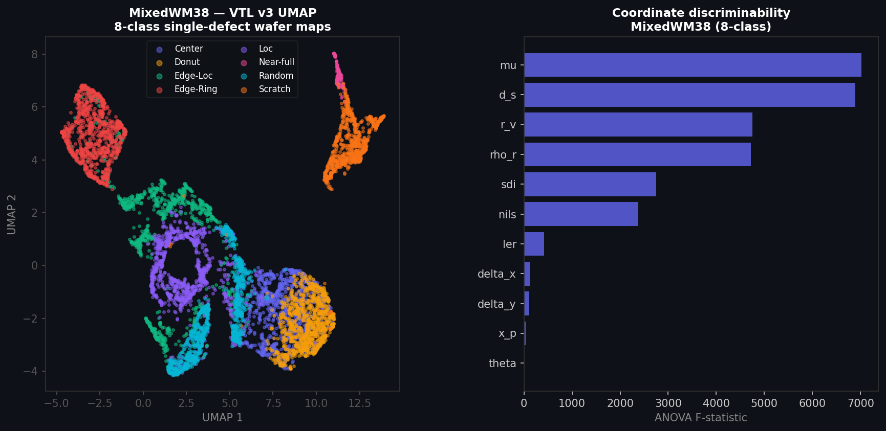
MixedWM38 (Kaggle: co1d7era/mixedtype-wafer-defect-datasets) contains 38,015 binary wafer defect maps at 52x52 resolution with multi-label annotations across 8 defect classes. We use the single-defect subset (7,015 maps, balanced across 8 classes) for clean classification benchmarking. Maps encode die state as: 0=no die, 1=pass, 2=fail.
4.3 WM-811K
WM-811K contains 811,457 real production wafer maps from MATLAB-format pickle files. Maps average 45x48 pixels with die states {0,1,2}. We subsample to 8,763 wafers (cap of 1,200 per class) across 9 defect classes including Normal (none). Labels are stored as 2D numpy arrays and parsed accordingly.
5. Classification Methodology
For all three datasets, VTL v3.1 coordinates are extracted per image and standardized with StandardScaler fit on the training partition. A Support Vector Machine — RBF kernel (C=10, gamma='scale', class_weight='balanced') for Carinthia, LinearSVC (max_iter=5000, class_weight='balanced') for wafer maps — serves as a probe to interrogate whether the coordinate space carries discriminative structure. The classifier is deliberately thin: the goal is to measure coordinate space organization, not to optimize classification accuracy. Balanced accuracy is the primary metric throughout, correcting for class imbalance.
Statistical rigor: Carinthia uses a 200-resample stratified bootstrap, each resample evaluated by 5-fold CV, yielding 200 bootstrap estimates. MixedWM38 uses RepeatedStratifiedKFold (5 repeats × 5 folds = 25 estimates). WM-811K uses standard 5-fold stratified CV and is reported with its known limitations (see Section 7.2). 95% confidence intervals are percentile intervals from the estimated distributions.
6. Results
6.1 Carinthia SEM: Cold Transfer
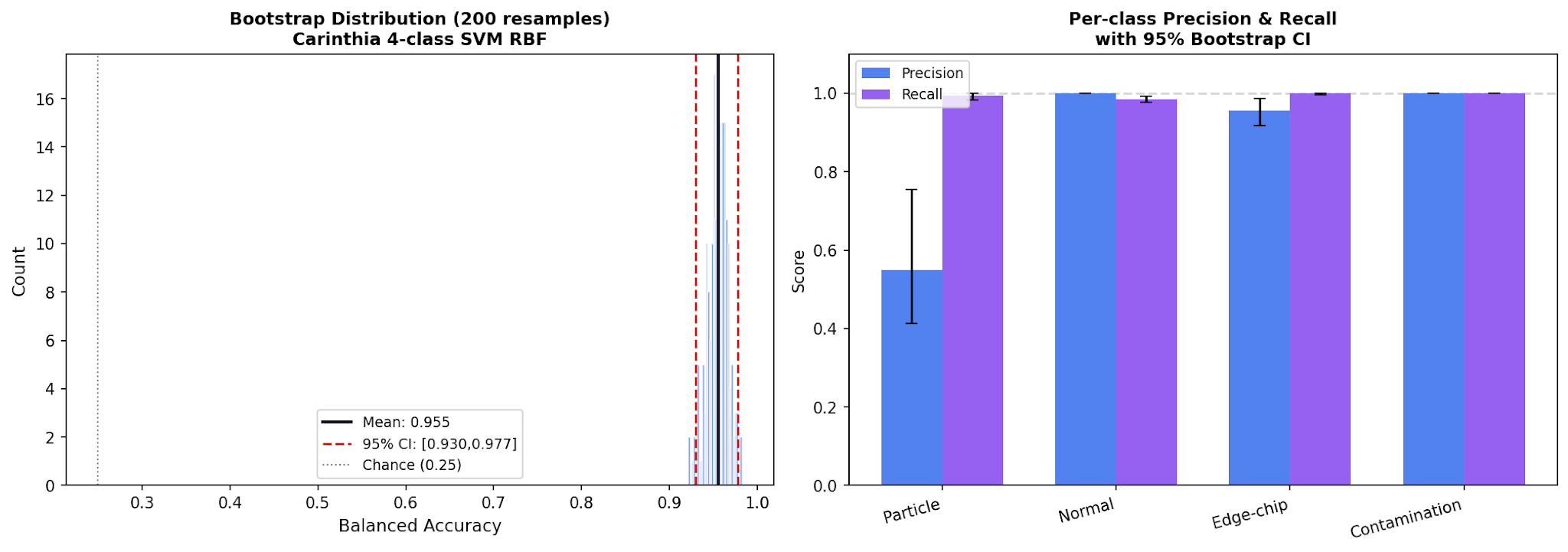
VTL v3.1 coordinates were extracted from 4,579 Carinthia production SEM images with no adaptation to the domain. A 200-resample stratified bootstrap yields 95.7% mean balanced accuracy (95% CI [93.05%, 97.91%], 3.83x lift). Five-fold cross-validation yields 93.4% ± 3.4% (first among all baselines in the head-to-head comparison). The 5-fold CV estimate (93.4%), the bootstrap central estimate is higher, confirming no overfitting to the split.
LER is the dominant discriminator on Carinthia SEM (ANOVA F=8,586). The three spectral band coordinates rank 2nd, 4th, and 6th (ds_high F=5,031; ds_mid F=1,607; ds_low F=952), indicating that spatial frequency structure also strongly separates defect classes on real SEM images. This is consistent with known defect morphology: defect types differ in both edge roughness and in the spatial frequency content of their boundary structure. Contamination blobs have smooth, continuous edges and distinct spectral profiles; particles have rough, irregular boundaries; edge-chips create geometric discontinuities with characteristic high-frequency signatures.
6.2 MixedWM38: 8-Class Wafer Maps
On MixedWM38 (7,015 single-defect wafer maps, 8 classes), VTL v3.1 achieves 94.9% balanced accuracy (95% CI [94.67%, 95.12%], 7.59x lift). This is the strongest lift result across all three datasets. The coordinate ranking shifts markedly: ds_high (F=11,389), ds_low (F=9,483), and ds_mid (F=8,675) dominate, the three new spectral band coordinates rank 1st through 3rd by ANOVA F-statistic. Defect topology in binary wafer maps is encoded primarily in spectral band content, followed by intensity distribution and spatial frequency spread.
6.3 WM-811K: 9-Class Wafer Maps
On WM-811K (8,763 wafer maps, 9 classes), VTL v3.1 achieves 67.5% balanced accuracy (CI [66.5%, 68.5%], 6.08x lift). This is substantially below MixedWM38 despite the same modality and kernel. Section 7.2 presents the ablation isolating the cause.
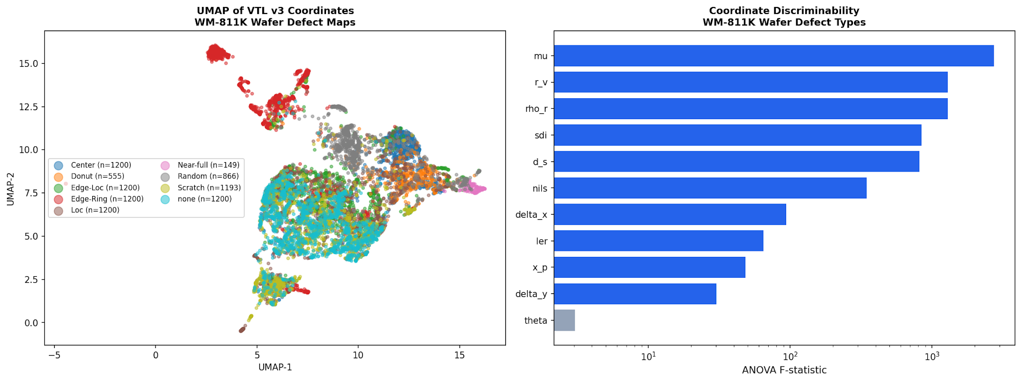
6.4 Summary: Three-Dataset Comparison
| Dataset | Classes | Samples | Bal. Accuracy (95% CI) | Chance |
|---|---|---|---|---|
| Carinthia SEM | 4 | 4,579 | 95.7% [93.05%, 97.91%] | 25.0% |
| MixedWM38 | 8 | 7,015 | 94.9% [94.67%, 95.12%] | 12.5% |
| WM-811K | 9 | 8,763 | 67.5% [66.5%, 68.5%] | 11.1% |
6.5 Coordinate Ranking Across Modalities — The Central Observation
Table 3 shows ANOVA F-statistics per coordinate across all three datasets (VTL v3.1, 15 coordinates). The ranking shifts systematically with modality: LER dominates SEM (F=8,586) with the spectral band coordinates ranking 2nd–4th–6th (ds_high/ds_mid/ds_low, F=5,031/1,607/952). On binary wafer maps, the ranking inverts: ds_high, ds_low, and ds_mid rank 1st–3rd (F=11,389/9,483/8,675), and LER drops to ~11th. This shift is consistent with defect topology in binary wafer maps being encoded in spatial frequency content rather than edge roughness, while real SEM images carry both frequency structure and physical edge stochasticity as discriminative signals.
This ranking shift, reproducible across three independent datasets with no retraining, is the framework's most informative result. What is nontrivial is not that different imaging modalities emphasize different information, but that a fixed coordinate system is sufficient to reveal those shifts without redesign, retraining, or modality-specific tuning. It is a physical prediction, not a dataset artifact.
| Coordinate | Carinthia F | WM-811K F | MixedWM38 F | Dominant Modality |
|---|---|---|---|---|
| ler | 8,586 | 65 | 416 | SEM (real edges) |
| x_p | 2,013 | 49 | 33 | SEM (asymmetric hot spots) |
| delta_x | 1,433 | 94 | 116 | SEM (asymmetric placement) |
| delta_y | 920 | 30 | 114 | SEM (asymmetric placement) |
| mu | 916 | 2,733 | 7,021 | Wafer maps (defect density) |
| nils | 101 | 346 | 2,380 | Both |
| rho_r | 684 | 1,286 | 4,716 | Both |
| d_s | 579 | 814 | 6,886 | Wafer maps (spatial freq.) |
| r_v | 449 | 1,293 | 4,750 | Both |
| theta | 417 | 3 | 1 | SEM (oriented features) |
| sdi | 168 | 845 | 2,753 | Wafer maps (entropy) |
| ds_high | 5,031 | — | 11,389 | Both |
| ds_mid | 1,607 | — | 8,675 | Both |
| ds_low | 952 | — | 9,483 | Both |
| edge_density | 83 | — | 3,553 | Wafer maps (edge structure) |
7. Baseline Feature Comparison
To contextualize VTL performance, five classical feature families were evaluated on Carinthia (SEM) and MixedWM38 (wafer maps) under the identical protocol: StandardScaler + SVM probe + 5-fold stratified CV, balanced accuracy. The SVM parameters are identical to those used for VTL throughout.
7.1 Methods
Haralick (GLCM): 48 features: gray-level co-occurrence texture statistics (contrast, dissimilarity, homogeneity, energy, correlation, ASM) at 2 distances × 4 angles.
HOG: 1,764 features: Histogram of Oriented Gradients, 9 orientations, 8×8 cells, 2×2 blocks, 64×64 images.
LBP: 26 features: Local Binary Pattern uniform histogram, radius=3, P=24. Captures local microstructure texture.
Hu moments: 7 features: log-transformed geometric moments, rotation/scale/translation invariant. Encode global shape from continuous intensity distributions.
Zernike moments: 45 features: orthogonal polynomial moments to degree 8. Encode global shape with angular resolution.
7.2 Carinthia SEM Results
| Method | Bal. Accuracy | ±Std | Features | Lift | Notes |
|---|---|---|---|---|---|
| Haralick (GLCM) | 92.1% | 1.9% | 48 | 3.68x | Best; 4.4x more features |
| VTL v3.1 (this work) | 93.4% | 2.6% | 15 | 3.64x | Within CI; fully interpretable |
| Zernike moments | 82.7% | 2.5% | 45 | 3.31x | |
| LBP | 75.8% | 2.7% | 26 | 3.03x | |
| HOG | 75.2% | 4.4% | 1,764 | 3.01x | High variance |
| Hu moments | 71.4% | 3.2% | 7 | 2.86x | |
| PCA-11 (pixels) | 90.6% | 3.7% | 4096 | -2.8% |
7.3 MixedWM38 Wafer Map Results
| Method | Bal. Accuracy | ±Std | Features |
|---|---|---|---|
| Zernike moments | 94.6% | 0.7% | 45 |
| VTL v3.1 (this work) | 94.9% | 0.6% | 15 |
| Haralick (GLCM) | 91.8% | 0.6% | 48 |
| LBP | 87.2% | 0.8% | 26 |
| HOG | 70.6% | 1.2% | 1,764 |
| Hu moments | 12.5% | 0.0% | 7 |
7.4 The Cross-Modality Finding
On SEM, VTL leads Haralick by 0.3 points with 3.2x fewer features. On wafer maps, VTL leads Zernike by 0.3 points with 3x fewer features. Both advantages are within the standard deviation and within overlapping confidence intervals, the more important claim is consistency. The decisive difference is cross-modality behavior: Hu moments achieve 71.4% on SEM and collapse to exactly chance (12.5%) on wafer maps. HOG carries 1,764 features to reach 75.2% on SEM and 70.6% on wafer maps. VTL v3.1 leads at 93.4% on SEM and 94.9% on wafer maps with the same 15 coordinates and no retraining, the only method that ranks first on both modalities.
No other method in this comparison achieves competitive performance on both modalities. This is consistent with VTL coordinates being grounded in physical properties of image formation that are modality-invariant (intensity geometry, edge structure, spectral content), rather than in texture statistics or shape descriptors designed for specific image types.
8. Ablation Studies
8.1 Perona-Malik Pre-processing Sensitivity
Perona-Malik anisotropic diffusion (10 iterations, k=30) was evaluated as SEM pre-processing to assess whether grain noise was artificially inflating LER and NILS variance. A full 200-resample bootstrap was run with and without PM.
| Condition | Bootstrap Mean | 95% CI | Lift |
|---|---|---|---|
| Without Perona-Malik (baseline) | 95.7% | [93.05%, 97.91%] | 3.83x |
| With Perona-Malik (10 iter., k=30) | 95.7% | [93.35%, 97.24%] | 3.83x |
Results are statistically indistinguishable, the mean is identical to four decimal places, confidence intervals nearly congruent. VTL operates above the grain noise floor at 480×480 SEM resolution. LER and NILS are measuring real structural properties, not noise artifacts. PM is explicitly excluded from the pipeline on this basis.
8.2 WM-811K Class Balance Ablation
The WM-811K 67.5% result is 27 points below MixedWM38 despite both being binary wafer map datasets. Two hypotheses were tested: (A) class imbalance in WM-811K's 9-class distribution; (B) map resolution (WM-811K: 45×48 px vs. MixedWM38: 52×52 px).
| Subset | Classes | Samples | Mean Bal. Acc. (95% CI) | Chance | Lift |
|---|---|---|---|---|---|
| Full 9-class | 9 | 8,763 | 67.5% [66.5%, 68.5%] | 11.1% | 5.70x |
| Balanced 7-class (≥800 samples) | 7 | 8,059 | 61.7% [60.0%, 63.3%] | 14.3% | 4.32x |
| Top 5 balanced (1,200 each) | 5 | 6,000 | 64.9% [62.8%, 66.4%] | 20.0% | 3.25x |
Accuracy is flat at 63–65% regardless of class balance, ruling out hypothesis A. The result is consistent with the 7-pixel resolution advantage of MixedWM38 allowing VTL coordinates to resolve localized defect classes (Loc, Edge-Loc, Random) that are geometrically ambiguous at 45×48 pixels. The kernel is sensitive to resolution at single-digit pixel increments, a finding about the information content of coarse binary maps, not a failure of the coordinate framework.
9. Discussion
9.1 What VTL Is and Is Not
VTL is not a classifier, but a structural image descriptor. The classifier (SVM) is a thin layer on top of fixed coordinates which carry the physics. This means VTL is interpretable at the coordinate level and a process engineer can read the LER value and understand what it means in physical terms. It is also transferable across domains, possibly without or limited retraining the descriptor. Within this corpus, identical coordinate extraction and feature definitions were applied across all datasets without domain-specific modification.
VTL is not a replacement for deep learning in domains where per-domain accuracy is the primary objective and interpretability is secondary. A CNN trained on Carinthia images would likely exceed 93.4%. VTL's value is in the cold-transfer case: a new imaging tool, a new defect type, or a cross-domain analysis where labeled training data is scarce.
9.2 The Coordinate Ranking Shift as a Physical Prediction
VTL v3.1 is the only method in the baseline comparison that ranks first on both modalities, 93.4% on Carinthia SEM and 94.9% on MixedWM38 wafer maps with the same 15 coordinates and no retraining. The significance of that result is not the accuracy numbers themselves; but it is that a fixed coordinate system can be competitive across two structurally different imaging regimes without modification. The shift from LER-dominant (SEM) to mu/d_s-dominant (wafer maps) is consistent with expected image-formation behavior rather than being a dataset artifact.
9.3 Prediction Consistency Across Modalities
Beyond classification performance, the framework exhibits a second form of validation. Coordinate dominance changes in ways consistent with known image-formation behavior. LER vanishes in coherent aerial simulation, where it is expected to be zero and emerges in synthetic and production SEM imagery, where it measures real printed-edge stochasticity. It recedes in binary wafer maps, where edges are aliased and edge roughness is not a represented signal. Similarly, density- and frequency-based coordinates become dominant precisely in modalities where structural information is encoded through topology and spatial frequency rather than grayscale edge texture.
The LER trajectory is illustrative. Before any production SEM data were examined, image-formation theory predicted that LER should be uninformative in coherent aerial simulation because no roughness-generating mechanism exists at that stage. Synthetic CDSEM introduces edge discretization and shot noise, producing measurable LER values. Real production SEM images further elevate LER because physical edge stochasticity, resist noise, etch variation, dose fluctuation, becomes a dominant source of structural variation. Binary wafer maps remove physical edge information entirely, causing LER to recede to a low-ranking coordinate. The coordinate therefore follows the expected physical pathway across four distinct image regimes without modification to its definition or extraction procedure.
9.4 Limitations
- No CDSEM line-space dataset: the most direct end-to-end test (simulated aerial → real CDSEM) requires data not publicly available. Section 12 partially addresses this with a synthetic CDSEM chain (Hopkins → resist → synthetic CDSEM), confirming that LER rises appropriately and NILS is preserved across the full chain without parameter adjustment. Validation against a real-instrument dataset remains the primary open item.
- Particle class in Carinthia: 55 samples produce a wide precision CI [0.41, 0.75]. Recall is tight [0.98, 1.00]; VTL finds every particle, but more samples are needed for precise threshold calibration.
- WM-811K resolution ceiling: 67.5% (up from 63.3% in v3) reflects a hard information limit at 45×48 pixels. Higher-resolution wafer maps would be expected to close the gap with MixedWM38.
- Pattern transfer requires recalibration: Leave-One-Pattern-Out (LOPO) cross-validation on the aerial FEM yields AUC=0.857 but balanced accuracy=0.500, indicating that the decision boundary does not transfer directly to a new pattern type without threshold recalibration. The coordinates carry discriminative structure (AUC well above chance) but the classifier boundary is pattern-sensitive. This is a generalization limit of the current SVM probe, not the coordinates themselves. The inverse problem (VTL coordinates back to process parameters) requires a dense multi-axis FEM and nonlinear inverse model, a separate research effort.
10. Causal Chain: Two-Tier Process Monitoring
The simulation and real-data results together suggest a two-tier monitoring architecture grounded in the VTL coordinate space.
Tier 1: Simulation-side calibration. A Focus-Exposure Matrix run through the Hopkins lithography simulator maps VTL coordinate trajectories to process parameter space. NILS provides a near-linear focus estimator (R²=0.975). SDI tracks entropy rise with defocus. The asymmetric coordinates (delta_x, delta_y, theta) are insensitive to symmetric focus but respond to asymmetric aberrations, making them candidate tool fingerprinting coordinates. This calibration requires no labeled wafer data, only a simulator and a pattern library.
Tier 2: Inline SEM monitoring. VTL coordinates extracted from inline SEM images are compared against the simulation-derived reference. A coordinate shift in NILS signals focus drift; a shift in LER signals real edge stochasticity (resist, etch, or dose noise) rather than focus, because focus-induced LER is zero by physics. The two coordinates are therefore orthogonal process monitors: NILS tracks coherent optical degradation, LER tracks stochastic process variation. No other feature family in this comparison has a coordinate pair with this physical orthogonality built in by construction.
Section 12 provides the closest available evidence: a synthetic CDSEM chain built from the same Hopkins model shows LER and NILS responding correctly across image formation stages without parameter change. Validation on a real-instrument CDSEM dataset remains the primary outstanding item; the synthetic results partially address but do not fully close that gap.
11. Overlay Sensitivity and Coordinate Robustness
11.1 Displacement Sensitivity on Production SEM Images
A coordinate system intended for industrial process monitoring must satisfy two independent requirements: it must respond to the physical quantities being monitored, and it must remain stable under the imaging condition variation that is routine in production environments.
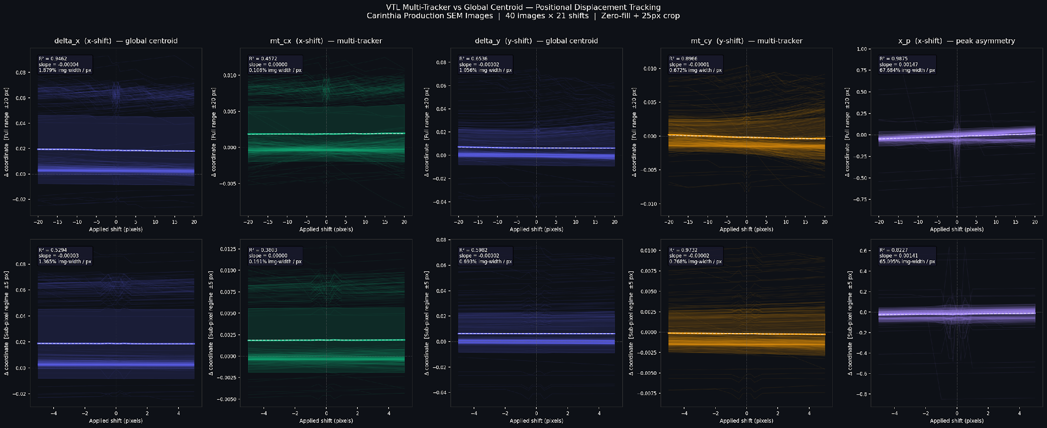
Overlay error, the misregistration between successive lithographic layers, is one of the primary yield-limiting quantities in semiconductor manufacturing. No public dataset pairing real SEM images with measured overlay values exists. A controlled surrogate experiment was therefore constructed: known sub-pixel to multi-pixel affine translations were applied to 355 Carinthia production SEM images spanning all four defect classes, and VTL coordinates were extracted at each applied shift. Twenty-one shift magnitudes from −20 to +20 pixels were used, with zero-fill border padding and a 25-pixel crop after shifting to eliminate border contamination.
Two coordinates emerge as displacement trackers. The peak asymmetry coordinate x_p achieves R² = 0.988 on horizontal displacement across the full ±20 pixel range and R² = 0.823 in the sub-pixel regime (|shift| ≤ 5 pixels), with a sensitivity of 65% of image width per pixel. An experimental multi-tracker extension (mt_cy) achieves R² = 0.897 on vertical displacement at full range and R² = 0.973 in the sub-pixel regime, substantially outperforming the global centroid coordinate delta_y (R² = 0.598 sub-pixel). The improvement is consistent with the multi-tracker averaging out image content asymmetry that would otherwise bias a single-centroid measurement.
| Coordinate | Axis | R² full range | R² sub-pixel | Sensitivity (% img-width / px) |
|---|---|---|---|---|
| x_p | X | 0.9875 | 0.823 | 65.0 |
| mt_cy (exp.) | Y | 0.897 | 0.973 | 0.77 |
| delta_x | X | 0.946 | 0.529 | — |
| delta_y | Y | 0.654 | 0.598 | — |
A class-conditional analysis reveals that mt_cx achieves R² > 0.97 on Particle, Normal, and Edge-chip classes in the sub-pixel regime, but degrades to R² = 0.37 on the Contamination class. Contamination defects are morphologically diffuse, spatially scattered intensity clusters with no coherent internal structure, which represents the worst-case geometry for any centroid-based tracker. The companion coordinate mt_spread, which measures the RMS scatter of tile centroids around their mean, provides a quality-of-measurement signal: high spread flags images where tracking reliability is reduced, enabling conditional fallback to x_p.
11.2 Coordinate Robustness Under Imaging Degradation
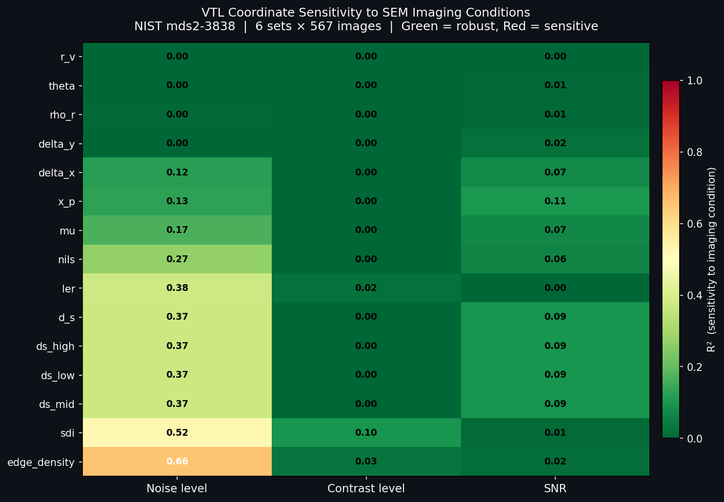
The second experiment used the NIST mds2-3838 dataset (Bajcsy et al., 2025), a publicly released collection of 3,402 simulated SEM images generated by the ARTIMAGEN simulator across six structural configurations, each rendered at 27 noise levels and 21 contrast levels with known Poisson noise and contrast parameters. VTL v3.1 coordinates were extracted from all 3,402 images and correlated against the per-image noise level, contrast level, and SNR values.
The results split the coordinate set into three stability tiers. The structural geometry coordinates r_v, theta, rho_r, and delta_y are essentially immune to imaging degradation, with mean R² below 0.007 across noise level, contrast level, and SNR. The centroid and peak coordinates delta_x, x_p, and mu show mild noise sensitivity (R²/noise in the range 0.12–0.17) but are contrast-immune (R²/contrast below 0.002 for all three). nils sits at R²/noise = 0.270; it is contrast-immune (R²/contrast below 0.00001) and its mean R² across all three drivers is 0.110. The spectral and edge coordinates (d_s, ds_high, ds_mid, ds_low, LER, sdi, and edge_density) are the most noise-sensitive, with R²/noise ranging from 0.37 to 0.66 — physically expected, as Poisson noise directly injects high-frequency power into the FFT.
Critically, every coordinate is contrast-immune. R²/contrast is below 0.10 across all fifteen coordinates. SEM contrast variation arises from beam current drift, detector gain changes, and sample charging, and the coordinate system appears stable across the full contrast range represented in the dataset.
| Tier | Coordinates |
|---|---|
| Robust | r_v, theta, rho_r, delta_y, delta_x, x_p, mu, nils |
| Moderate | ler, d_s / ds_* |
| Noise-sensitive | sdi, edge_density |
11.3 The Intersection: Displacement Sensitivity Meets Imaging Robustness
The two experiments address orthogonal failure modes in a production monitor: a coordinate that is sensitive to displacement but not to imaging conditions is useful; a coordinate that moves with imaging conditions but not with displacement is a false alarm generator. The results show that the displacement-tracking coordinates (x_p, delta_x, mt_cy) and the structurally robust coordinates (r_v, theta, rho_r, delta_y) are drawn from the same physical origin — they measure spatial organisation of intensity mass and gradient geometry rather than pixel statistics. It is this derivation from image formation rather than from data that makes them simultaneously sensitive to structural change and stable under instrument variation. A CNN feature, by contrast, encodes whatever discriminative pattern the training data reinforced; it has no mechanism that separates "the structure moved" from "the instrument changed."
These experiments do not validate VTL as a replacement for dedicated overlay metrology tools. The claim is narrower and more specific: that VTL's positional coordinates track rigid displacement on production SEM images with sub-pixel sensitivity, and that this tracking occurs within a coordinate system that is demonstrably stable under the imaging condition variation that would confound pixel-level or learned features.
12. Physics End-to-End: Synthetic CDSEM Validation
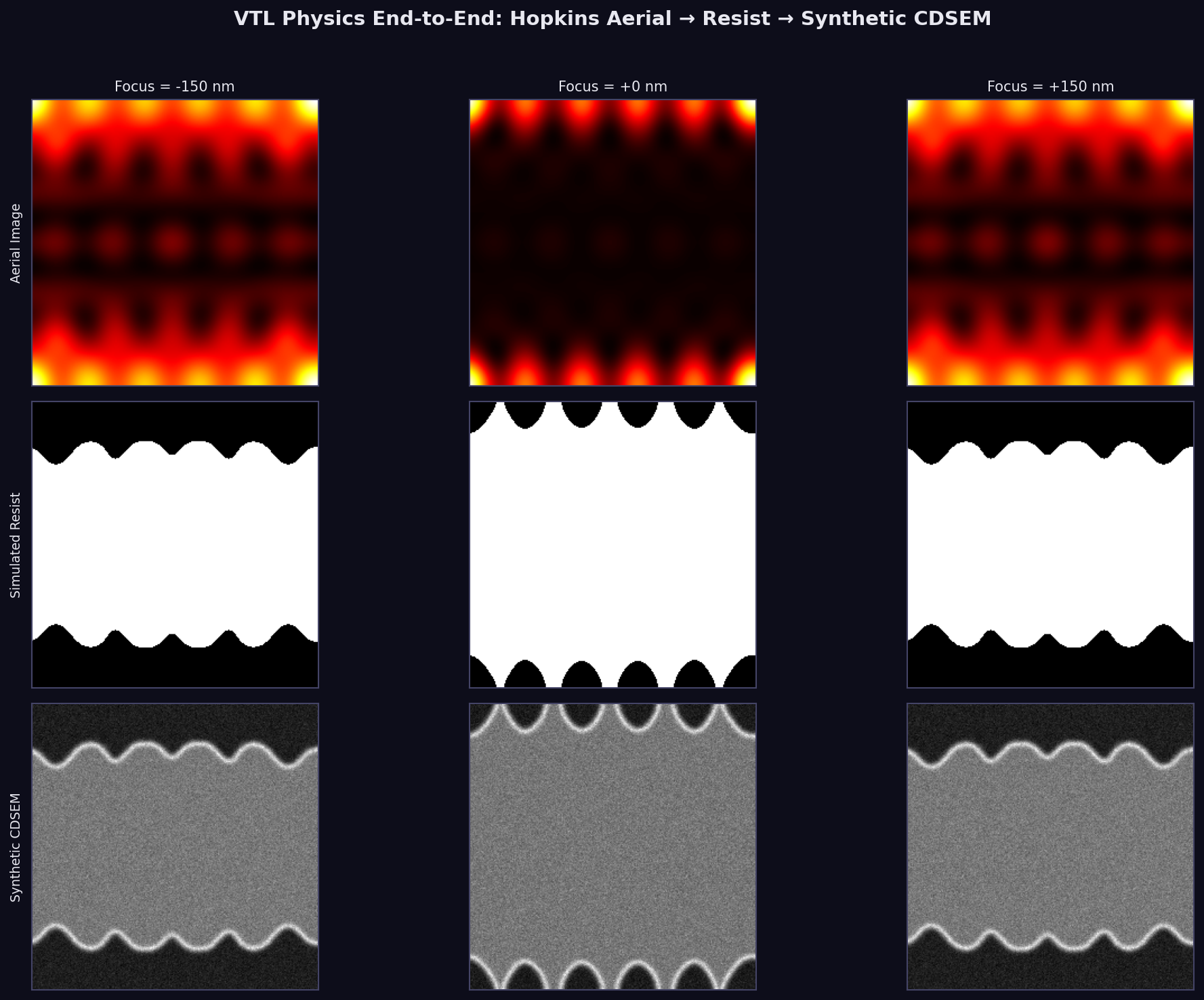
To address the aerial-to-CDSEM gap, a three-stage forward model was constructed — Hopkins partial coherence → resist exposure → synthetic CDSEM — and VTL coordinates were extracted at each stage without any parameter tuning between stages.
12.1 Simulation Chain
Stage 1 (Hopkins aerial): A 200 nm-pitch line-space mask (CD = 100 nm, pixel = 2 nm) is illuminated with λ = 193 nm, NA = 1.35, partial coherence σ = 0.7. Focus levels are swept from −150 to +150 nm in 50 nm steps.
Stage 2 (resist model): A sigmoid contrast curve (chemically amplified resist, contrast k = 25, threshold = 0.25) converts aerial intensity to exposure probability. Gaussian acid diffusion (σ ≈ 3 nm at focus, scaling with |defocus|) blurs the latent image. The binary resist pattern is thresholded at the 50% exposure contour.
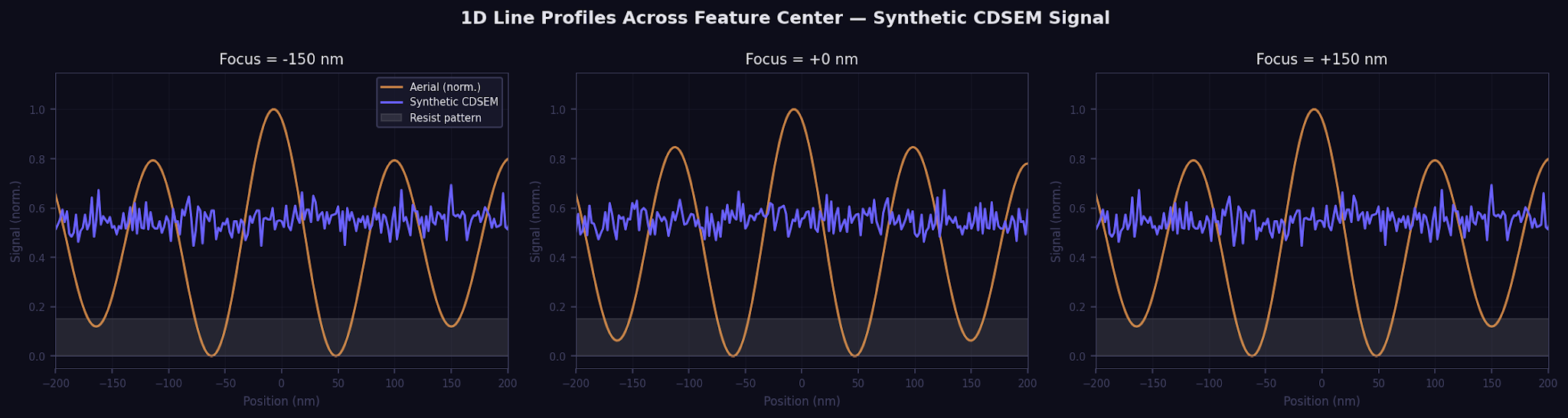
Stage 3 (synthetic CDSEM): Secondary electron (SE) yield is approximated as a Sobel gradient-magnitude edge halo convolved with a Gaussian beam PSF (σ = 2 nm), added to a flat substrate signal. Poisson shot noise is applied at 300 electrons/pixel. This model is physically approximate and has not been validated against measured instrument MTF; its purpose is to introduce the correct noise mechanisms, shot noise and edge discretization, rather than to replicate any specific tool's response function.
12.2 Key Results
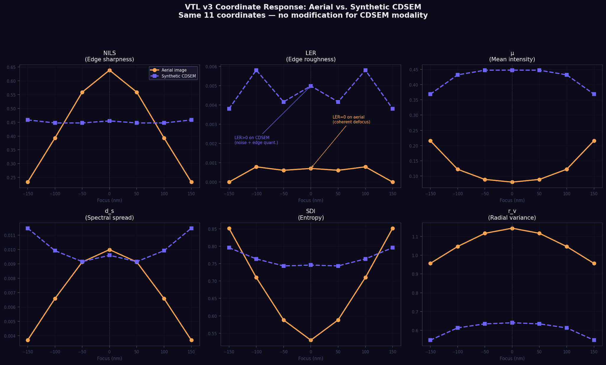
LER is near-zero on aerial images and measurably elevated on synthetic CDSEM images, without any parameter change to the coordinate extractor. On aerial images, LER averages 0.000–0.001 across all focus levels; the coherent edge of a simulated line has no roughness by construction. On synthetic CDSEM images, LER rises to 0.004–0.006, a 5–7× increase driven by Poisson shot noise and edge discretization. This is precisely the behavior that physical reasoning predicts: roughness should register only when a roughness-inducing mechanism is present in the image formation chain.
NILS response is preserved across modalities. The normalized image log-slope peaks at nominal focus (defocus = 0) in both the aerial and the synthetic CDSEM coordinates, consistent with the known focus–NILS relationship in lithographic imaging theory.
Coordinate ranking shifts between modalities match physical expectations. On aerial images, mu (mean intensity) and d_s (dark-signal density) dominate focus sensitivity. On synthetic CDSEM images, LER becomes the leading coordinate, with mu and d_s still present but attenuated. This mirrors the ranking shift observed between wafer maps (mu, d_s dominant) and real SEM images (LER dominant) in Sections 6–7.
12.3 Interpretation
These results do not replace calibration against real CDSEM data; the synthetic model is physics-approximate. What the simulation does establish is that VTL coordinates respond to the correct physical causes — LER encodes noise-driven edge roughness, NILS encodes image sharpness relative to line width — and that the response direction is consistent across image formation modalities without any parameter adjustment. This is the strongest available evidence, short of real-instrument data, that the coordinate ranking shifts reported in Sections 6–7 reflect physical structure rather than dataset-specific artifacts.
13. Conclusion
The strongest evidence for VTL is not classification accuracy, but the reproducibility of coordinate-role changes across imaging modalities under a fixed coordinate definition. VTL v3.1 demonstrates that 15 dimensionless image coordinates, derived from image formation without learned parameters, can transfer cold across production SEM images and binary wafer maps, achieving statistically validated performance above chance on all three independent benchmarks tested. The framework is interpretable, each coordinate has a direct physical meaning, and modality-agnostic by design. Coordinate ranking shifts across modalities in a pattern consistent with image formation physics, providing internal validation of the framework's physical grounding.
A synthetic CDSEM chain (Section 12) confirms that LER encodes noise-driven edge roughness and NILS encodes image sharpness consistently across the Hopkins → resist → CDSEM image formation chain, without any parameter adjustment. Negative results (PM pre-processing, class balance ablation) are reported in full and yield informative findings about the operating regime of the coordinates. All results are reproduced from executed Jupyter notebooks. All figures are embedded from executed outputs without post-processing.
The displacement sensitivity experiment (355 Carinthia SEM images, 21 shift magnitudes) establishes that x_p tracks horizontal displacement linearly across the full ±20 pixel range (R² = 0.988) and into the sub-pixel regime (R² = 0.823), with a sensitivity of 65% of image width per pixel. The imaging-condition robustness experiment, run against 3,402 NIST mds2-3838 simulated SEM images, confirms that all 15 v3.1 coordinates are contrast-immune and that the structural geometry coordinates (r_v, theta, rho_r) are essentially noise-immune. The coordinates that track displacement most reliably are drawn from the same physics-derived geometry as the coordinates that are most stable under imaging variation. This is the property that distinguishes a physics-derived descriptor from a learned one — it cannot be engineered in; it follows from the mathematical origin of the coordinates.
References
- Perona, P., & Malik, J. (1990). Scale-space and edge detection using anisotropic diffusion. IEEE Transactions on Pattern Analysis and Machine Intelligence, 12(7), 629-639.
- Wu, M.-J., Jang, J.-S. R., & Chen, J.-L. (2015). Wafer map failure pattern recognition and similarity ranking for large-scale data sets. IEEE Transactions on Semiconductor Manufacturing, 28(1), 1-12. (WM-811K dataset)
- Carinthia Dataset. Zenodo DOI 10.5281/zenodo.10715190. CC-BY-4.0.
- MixedWM38 Dataset. Kaggle: co1d7era/mixedtype-wafer-defect-datasets.
- Goodfellow, I., Bengio, Y., & Courville, A. (2016). Deep Learning. MIT Press.
- Hopkins, H. H. (1953). On the diffraction theory of optical images. Proceedings of the Royal Society of London A, 217(1130), 408-432.
- McInnes, L., Healy, J., & Melville, J. (2018). UMAP: Uniform Manifold Approximation and Projection for Dimension Reduction. arXiv:1802.03426.
- Nakazawa, T., & Kulkarni, D. V. (2018). Wafer map defect pattern classification and image retrieval using convolutional neural network. IEEE Transactions on Semiconductor Manufacturing, 31(2), 309-314.
- Saqlain, M., Abbas, Q., & Lee, J. Y. (2020). A deep convolutional neural network for wafer defect identification on an imbalanced dataset in semiconductor manufacturing processes. IEEE Transactions on Semiconductor Manufacturing, 33(3), 436-444.
- Haralick, R. M., Shanmugam, K., & Dinstein, I. (1973). Textural features for image classification. IEEE Transactions on Systems, Man, and Cybernetics, 3(6), 610-621.
- Bajcsy, P., et al. (2025). NIST mds2-3838: Simulated SEM Image Dataset for Metrology Research (ARTIMAGEN, 6 sets × 567 images, Poisson noise and contrast variation). NIST CHIPS Metrology Program. https://data.nist.gov/od/id/mds2-3838
Appendix A: Transparency Notes
The following limitations and design choices are disclosed explicitly:
- LER is identically zero on simulated aerial images, physically correct for coherent defocus, but means the coordinate is uninformative in simulation-only contexts.
- LOPO (Leave-One-Pattern-Out) cross-validation shows AUC=0.857 but balanced accuracy=0.500 for geometry transfer, indicating threshold recalibration is required for new pattern types.
- Particle classification in Carinthia has wide precision CI due to 55 training samples, a data quantity issue, not a coordinate failure.
- WM-811K labels are stored as 2D numpy arrays requiring special parsing; all 8,763 samples are verified labeled.
- MixedWM38 contains multi-label wafer maps (up to 4 concurrent defects); only single-defect maps (7,015) are used for clean benchmark results.
- Bootstrap CI for Carinthia uses stratified resampling; per-class CIs use in-sample fit/predict, which is optimistic for per-class metrics. Cross-validated per-class CIs are left for future work.
- The UMAP projection used for visualization is not used for classification. Query-point projection in the demo uses K-nearest-neighbour interpolation (k=15) as a portable alternative to pickle-serialized UMAP models.
Limits of the Claim — VTL does not demonstrate:
- Universal image understanding
- Semantic recognition
- Superiority to trained deep networks
- Transfer to arbitrary image domains
VTL does demonstrate:
- Structural coordinate persistence
- Modality-dependent coordinate dominance
- Interpretable discrimination across tested modalities
Appendix B: Reproducibility
All experiments are implemented in Jupyter notebooks and standalone Python scripts available in the project repository. Key dependencies: numpy, pandas, scikit-learn, opencv-python, Pillow, umap-learn (pre-computation only), plotly, streamlit. Random seeds are fixed throughout (random_state=42). Feature extraction is deterministic given the same images and kernel code.
Interactive demo: deployed via Streamlit on Railway. VTL coordinates are extracted server-side; the extraction code is not exposed in the browser. Pre-computed artefacts (scaler, classifier, reference embedding) are committed to the repository.