We present Ω, the mean pairwise disagreement among N physically independent structural reads of a field, and demonstrate that the pre-arrival seismic Ω signal decomposes into three separable layers: a floor (~0.040) present on quiet days with no earthquake; an ambient timing layer (+0.060) recovered by FK beamforming on pre-arrival data without earthquake priors; and a geometric amplification layer (+0.069) added by event-geometry-informed arrival-time picks. The geometric stagger does not create the pre-arrival elevation, it amplifies a genuine ambient signal approximately 2-fold. The decomposition is reproducible across five events spanning winter and summer, NW and SE source directions, and magnitudes Mw 7.0–9.0.
The pre-arrival ambient field has coherent directional timing structure detectable without earthquake priors. Data-driven arrival-time picks (no source location, no travel-time model) produce pre-arrival Ω = 0.100 vs P-window Ω = 0.075 (Cohen d = 1.78, 4/5 events). The floor without any directional stagger (~0.040) is indistinguishable from a quiet day. Standard semblance fails to discriminate pre-arrival from P-window on a continental array (wrong direction). Data-driven Ω outperforms mean pairwise cross-correlation (d = 0.17) and same-image Ω (d = 1.05) under matched conditions. The discriminating power gain from physical independence of observables is 6.9× over correlated transforms; the geometric amplification layer is separable from this independence gain.
FK beamforming failures on compact IMS-class arrays (15 cases, 4 arrays, 2 continents) provide the operational consequence: in twelve cases the direct P-wave was present and physically real yet did not win. SNR does not separate the three structural failure families; station-removal robustness does. The same operational symptom emerges from pre-existing ambient dominance, fragile knife-edge coherence, and a robust coherent competitor coupled to the P-wave onset. Coherence and correctness are separable variables. When the field supports multiple simultaneous coherent organizations, a single-answer instrument will pick one, and may pick the wrong one.
In the Japan 2021 Mw 7.1 earthquake recorded at PDAR (Idaho, USA), the direct P-wave was present at 71% of FK beamformer peak power. The instrument chose the peak. The peak corresponded to a back-azimuth of 105.3°. The earthquake was at 45.6°. The error was 59.7°.
The field was not missing a valid answer. It contained one. The instrument found a different one instead. Standard signal-to-noise ratio did not flag this: the direct P was energetically detectable, present above noise, physically real. The instrument was not starved of signal. It was choosing among signals, and it chose wrong.
This situation, a correct answer present but not dominant, arises whenever a measurement field contains multiple simultaneous coherent organizations. Standard seismic processing assumes that signal rises above a stochastic background, so signal-to-noise is the appropriate quality metric. When the background is not stochastic but contains its own coherent structure, that assumption breaks. Coherence and correctness become separable. A field can be highly organized around the wrong answer.
This paper asks a different question from existing seismic processing methods. Not: where is the signal? But: how many coherent answers is the field currently supporting? We present a measurement, Ω, the pairwise disagreement among physically independent structural reads of a field, that quantifies this directly. We demonstrate it on two teleseismic events recorded across the USArray Transportable Array, and connect it to FK beamforming failures on compact IMS-class arrays that provide twelve empirical examples of what happens when a single-answer instrument commits to a field that has not yet collapsed to one dominant organization.
Signal-to-noise ratio measures energetic dominance over a stochastic background. Semblance measures waveform similarity across array stations. FK beamforming measures phase coherence across stations at a given slowness and back-azimuth. Each of these answers the question: how strong is the signal relative to what surrounds it? None of them ask: how many competing structures does the field currently support?
The distinction matters because seismic fields routinely contain multiple simultaneous coherent organizations. Seismologists name them: microseismic noise, teleseismic coda from other events, surface wave trains, scattered arrivals, multipath energy. Naming them is not the same as measuring the degree to which they compete with the signal of interest. Existing quality metrics treat the non-signal components as a background to be overcome. We treat them as organizations to be measured.
Section 2 defines Ω and establishes the independence requirement, the finding that the discriminating power of Ω depends on the degree of physical independence among the theories reading the field, and that this degree is itself measurable. Section 3 describes the data and experimental design. Section 4 presents the three-window result: Ω collapses during the P arrival and expands again, in both events, across opposite source geometries. Section 5 presents the pairwise decomposition identifying what the pre-arrival plurality is made of. Section 6 presents FK beamforming failures as twelve empirical examples of the operational consequence: a single-answer instrument encountering a field that has not collapsed. Section 7 discusses the coherence/correctness separation and its implications. Section 8 concludes.
Given any spatially sampled field and N theories for locating the field's structural center, Ω is the mean pairwise Euclidean distance between the N centroid estimates in normalized field coordinates:
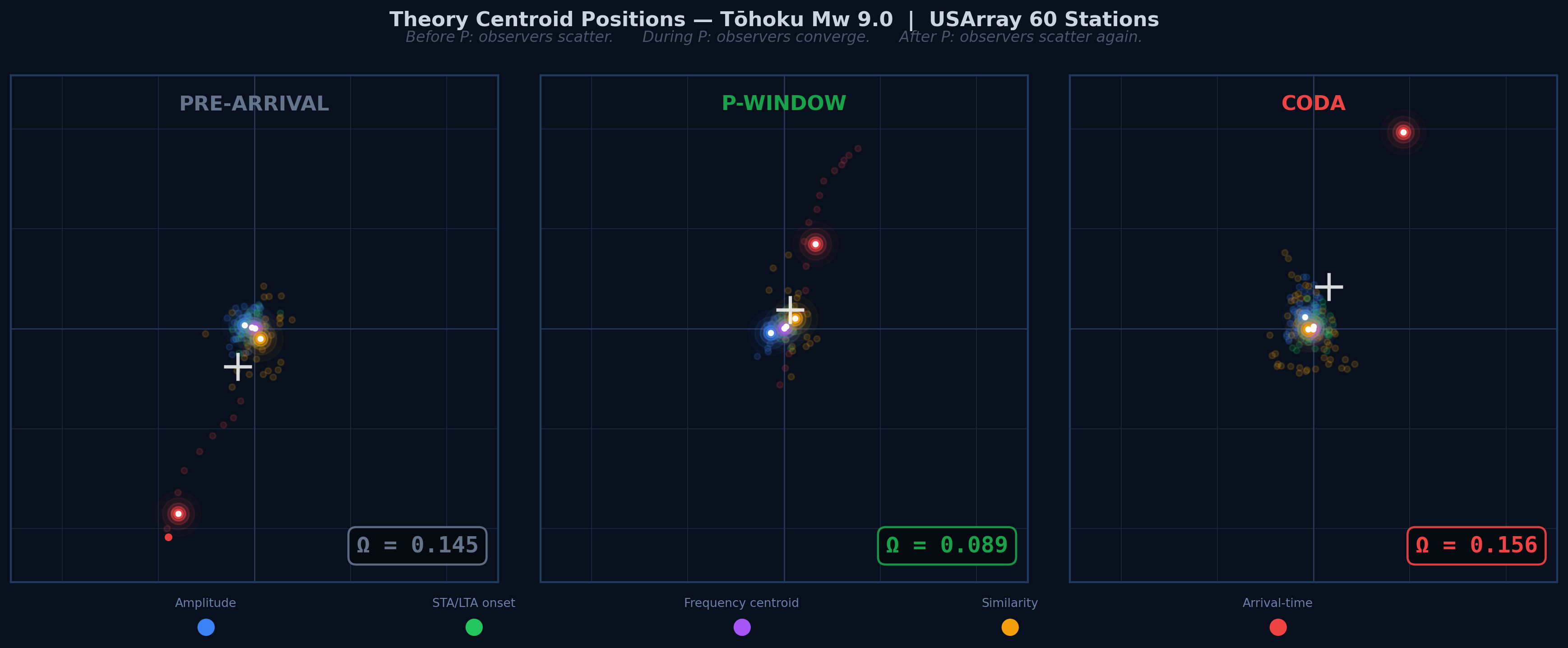
where each ci is a centroid position in [−0.5, 0.5]² normalized image space. Ω = 0 when all theories agree: the field has a single well-defined structural center. Ω near 0.5 when theories maximally scatter: the field supports no dominant organization or supports multiple organizations that pull in different directions.
The instrument is named Parallax for the principle it operationalizes: the apparent displacement of an object viewed from different positions. The difference between the views is the measurement. When the views converge, the object is well-located. When they diverge, independent observers are finding different spatial centers, not because of bias, but because the field is organized differently for different physical quantities simultaneously.
The central methodological finding of Stage 1: the discriminating power of Ω depends on whether the N theories read genuinely different physical observables, not different mathematical transforms of the same input.
In the original formulation, five theories were applied to one interpolated amplitude image: global intensity-weighted centroid, multi-tracker tile-grid centroid, spectral residual saliency, fine-scale Difference-of-Gaussians, and coarse-scale Difference-of-Gaussians. These five theories produce different functions of the same input surface. When the amplitude image shifts, all five theories shift together. Their disagreement reflects mathematical transform diversity, not physical field disagreement. The mean pairwise separation between P-window and coda under this formulation was 0.004.
Replacing those five transforms with five observables reading genuinely different physical properties of the wavefield, amplitude, STA/LTA onset, dominant frequency, inter-station similarity, and arrival-time geometry, produced a mean P/coda separation of 0.137. The increase is 6.9× under matched (data-driven) conditions. Event-geometry stagger adds a further amplification layer. Both gains are real; this paper reports 6.9× as the independence gain from physical independence alone. The gain came entirely from reading different physics.
This result can be stated as a principle: the discriminating power of Ω scales with the degree of physical independence among the input theories. Independence is quantifiable: the mean off-diagonal absolute correlation of the observable matrix (I) measures it directly. When I is high, theories share input and Ω measures transform diversity. When I is low, theories read separate physical channels and Ω measures genuine field disagreement.
Each of the five observables places a geographic centroid by weighting station positions according to a station-level measurement derived from a distinct physical property of the waveform:
| Observable | Weight per station | Physical property read |
|---|---|---|
| Amplitude | 90th-percentile absolute amplitude in window | What is energetically loud right now |
| STA/LTA onset | Short-term / long-term average ratio at window | What is emerging, onset contrast |
| Frequency centroid | Spectral center of mass, 0.5–2 Hz band | Dominant frequency character |
| Inter-station similarity | Zero-lag correlation with array stack | Coherence with the collective wavefield |
| Arrival-time | exp(−|t − tpick| / τ), τ = 20 s | Where the wavefront arrived first |
A sixth observable, polarization centroid, weighted by radial fraction of horizontal energy from BHN and BHE components, was computed for the Tōhoku event using all 60 stations and confirmed to read a physically distinct property with a separate centroid trajectory. Results with and without the polarization channel are reported where relevant.
The instrument has two distinct operating regimes determined by the amplitude normalization choice. Using raw peak amplitude per station, the primary discriminator between P-window and coda is σ(Ω): the temporal stability of the centroid constellation. Using SNR-normalized amplitude (peak divided by pre-event noise RMS), the primary discriminator becomes mean Ω: the spatial coherence of the field at a given moment. The two regimes answer different questions. Raw amplitude asks: is the field's organizational structure stable over time? SNR-normalized amplitude asks: is the field spatially organized right now? This paper uses raw amplitude and reports σ(Ω) alongside mean Ω.
The Parallax amplitude centroid requires network aperture at least ten times the dominant signal wavelength (aperture/λ > 10) to measure wavefield heterogeneity rather than site amplification patterns. Below this threshold, near-surface geology dominates amplitude variation across the array, and the centroid becomes event-invariant: it points to the same direction regardless of source azimuth. At PDAR (3.63 km aperture, λ ≈ 8 km at 1 Hz, aperture/λ ≈ 0.45) and TXAR (4.45 km, aperture/λ ≈ 0.56), the centroid pointed to 281–283° for both Tōhoku (true 46°) and Chile (true 334°): event-invariant, reading geology not wavefield. The USArray Transportable Array (aperture ~2000 km, aperture/λ ≈ 250) operates well within the envelope.
This boundary condition is not a failure of the instrument. It defines the scale at which the question changes. FK beamforming operates at the sub-wavelength compact-array scale using phase delays and is the appropriate direction-finding instrument there. Parallax operates at the continental-array scale using spatial field organization. They are complementary tools at different spatial scales asking different questions of the same phenomenon. The FK failures in §6 are analyzed precisely because Parallax cannot be deployed on compact arrays, but they show what happens when a single-answer instrument commits in a field that has not resolved to one dominant organization. The argument is motivational: pre-commitment field-state assessment using an independent instrument would identify when that commitment is risky. Parallax demonstrates that such assessment is possible in principle at continental scale. What form it would take at compact-array scale, using observables appropriate to that geometry, is a distinct engineering problem that Section 6 frames but does not solve.
The independence score I of an observable set is defined as the mean absolute off-diagonal Pearson correlation of the N observable centroid timeseries across all array timesteps. Low I indicates genuinely independent theories; high I indicates theories that share input and measure transform diversity rather than field disagreement.
| Theory set | N theories | I score (mean off-diag |r|) | Ω P/coda separation | Gain vs baseline |
|---|---|---|---|---|
| Five same-image amplitude transforms | 5 | ~0.85–0.95 (by construction: shared input) | 0.004 | baseline |
| Five physically independent observables | 5 | 0.159 | 0.137 (geo-stagger); 0.0665 (data-driven) | 6.9× (independence); ~34× (independence + geo amplification) |
| Six observables (+ polarization) | 6 | 0.159 (BHZ theories); polarization partially independent | 0.116 | 29× |
The highest remaining correlation among the six independent theories is between arrival-time and polarization (|r| = 0.436): both track wavefront geometry, though from physically distinct sensors (timing vs particle motion direction). All other off-diagonal correlations are below 0.26. The five-observable set (without polarization) is used as the canonical dataset for this paper because it has the cleanest independence profile and is the bootstrap-validated set.
During instrument development, an unexpected directional coordinate emerged from adversarial testing. Encoding STA/LTA-picked P arrival times across the array as a spatial intensity image, earliest arrivals brightest, latest arrivals darkest, and applying VTL theta (intensity-weighted dominant gradient orientation) to that image recovers the wave propagation back-azimuth without using the geographic source location, a velocity model for the full propagation path, or any phase-delay measurement.
Results for both events using non-circular STA/LTA picks (no geometric assumptions after the initial ±25 s search window):
| Method | Tōhoku baz error | Chile baz error | Circular? |
|---|---|---|---|
| FK beamforming (PDAR) | 46.3° | 4.5° | No (no model used) |
| FK beamforming (TXAR) | 66.5° | 1.5° | No |
| θ_mv (STA/LTA independent picks) | 6.6° | 3.5° | No |
| Plane-wave slowness fit (observed picks) | 12.9° | 10.2° | No |
θ_mv outperforms FK on Tōhoku by nearly an order of magnitude (6.6° vs 46.3° at PDAR) despite using a simpler input, a static spatial image of arrival timing, not waveform phase coherence. For Chile, where FK succeeds, θ_mv performs comparably (3.5° vs 1.5–4.5°).
The θ_mv result is not presented as an operational replacement for FK beamforming. It is a proof of concept that the information needed to recover the correct back-azimuth was present in the arrival-time geometry of the wavefield even when FK chose the wrong answer. The arrival-time centroid, which drives pre-arrival Ω in the pairwise decomposition, and the θ_mv coordinate are both manifestations of the same physical signal: the spatial pattern of wavefront timing across the array. The instrument can read it. FK on compact arrays, in the failure regime, cannot.
θ_mv is robust to station count reduction: errors remain below 7° at N = 25 and reach 7.0° [95% CI: 0.7–15.8°] only at N = 10. At N = 60, the 95% CI collapses to a point (single deterministic result), confirming the estimate is stable across the full array.
| Tōhoku 2011 | Chile 2010 | |
|---|---|---|
| Date/time | 2011-03-11T05:46:24Z | 2010-02-27T06:34:12Z |
| Magnitude | Mw 9.0 | Mw 8.8 |
| Location | 38.3°N, 142.4°E | 35.9°S, 72.7°W |
| Back-azimuth from array center | 314.6° | 156.7° |
| Distance | 9097 km | 9009 km |
| P travel time | ~19.0 min | ~18.8 min |
The two events arrive from source geometries 158° apart, providing the maximum available contrast in source direction for a single fixed array. Both are among the best-recorded teleseismic events in the USArray archive, with high SNR across all 60 stations.
60 USArray Transportable Array stations were selected in a compact region spanning 34–48°N, 88–115°W (array center approximately 41°N, 102°W). BHZ channel, 0.5–2 Hz bandpass, instrument response not removed, resampled to 1 Hz. 20-second sliding windows at 5-second step. Station coordinates from EarthScope FDSN metadata.
The following predictions were stated before any data were examined:
All five predictions were confirmed. Results are reported against locked predictions without post-hoc revision.
Pre-arrival window: all timesteps before P-window onset. P-window: P-window onset − 20 s to P-window onset + 60 s. Coda window: P-window onset + 120 s to P-window onset + 400 s. For Tōhoku (P predicted at t = 180 s from waveform start): pre-arrival t < 175 s (N = 33), P-window 175–205 s (N = 7), coda 240–375 s (N = 28). For Chile (P offset = 180 s): pre-arrival t < 160 s (N = 30), P-window 160–240 s (N = 17), coda 300–580 s (N = 57).
The results in §4.1–4.2 use event-geometry-informed arrival-time picks, the original pipeline in which each station's pick search window is centered on its predicted P-arrival time from the source location. This produces the largest pre-arrival Ω values and the clearest three-window structure. Section 5c then applies a systematic ablation that separates this signal into three independent components: a floor present without any directional information, a genuine ambient timing layer recoverable from pre-arrival FK beamforming alone, and a geometric amplification layer from the event-geometry prior. Readers should treat the numbers below as the full event-geometry signal, with the decomposition in §5c showing how much of that signal is ambient-field-driven versus prior-driven.
| Window | N | Mean Ω | Std Ω | Cohen d vs P-window | MW p vs P-window |
|---|---|---|---|---|---|
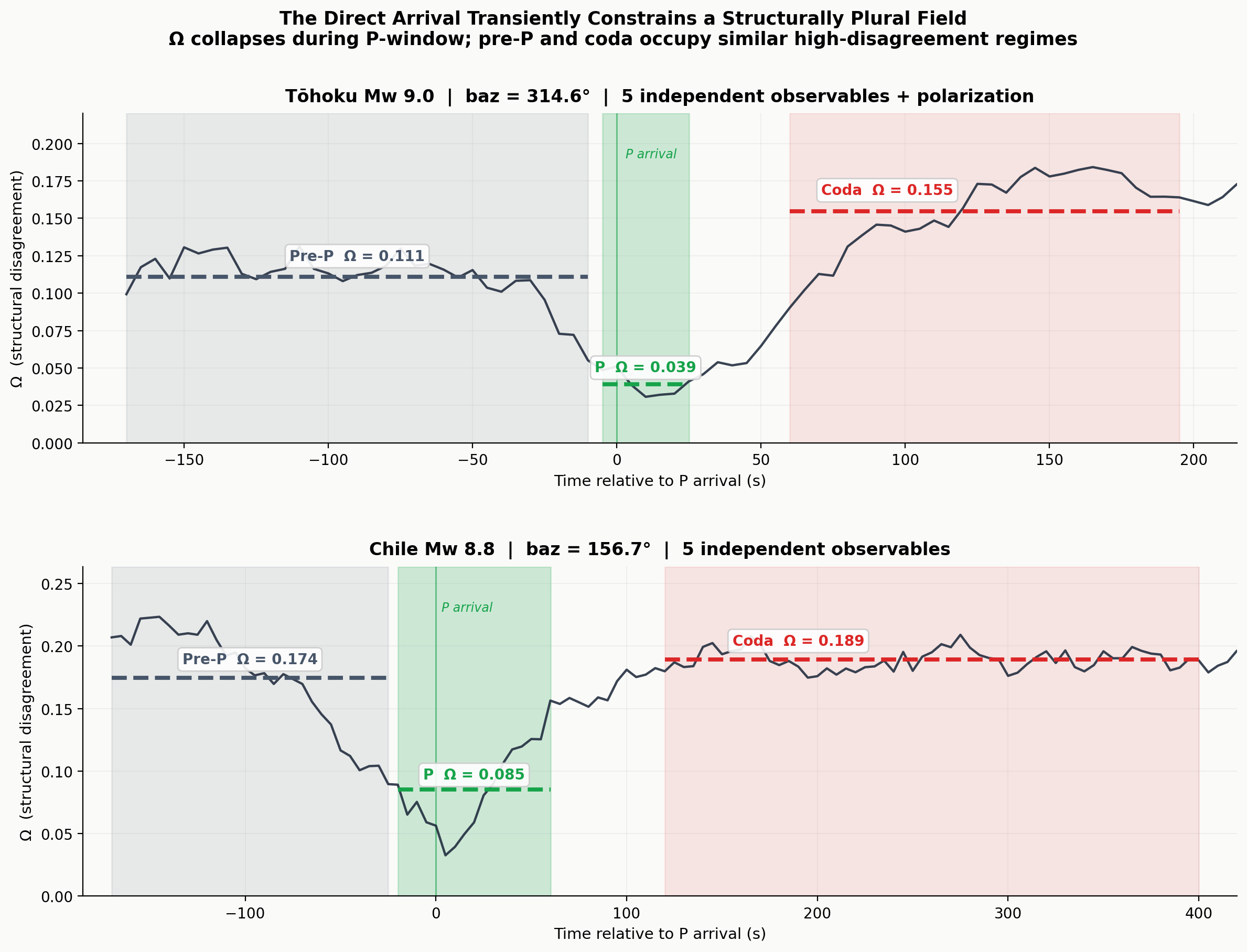
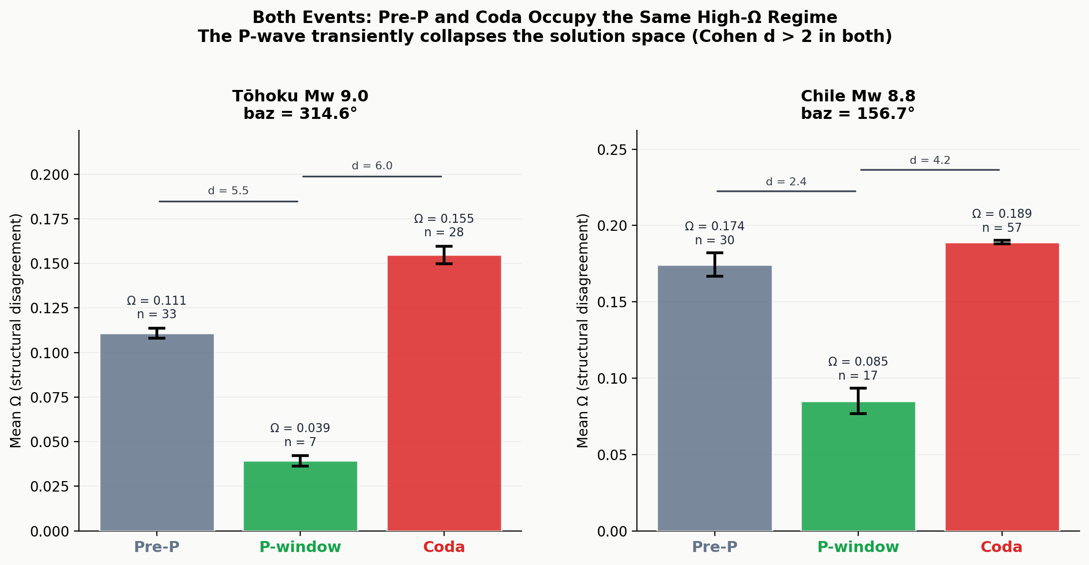
| Pre-arrival | 33 | 0.111 | 0.017 | 5.53 | < 0.0001 |
| P-window | 7 | 0.039 | 0.008 | — | — |
| Coda | 28 | 0.155 | 0.026 | 6.04 | < 0.0001 |
Pre-arrival vs coda: Cohen d = 2.01, p < 0.0001. The coda is more disordered than the pre-arrival baseline, consistent with scattered energy added by the earthquake to the ambient field. Bootstrap validation on event-geometry Ω (N = 10,000 block bootstrap, stage1_omega_6obs.pkl): σ(Ω) ratio 3.30× [95% CI: 1.63–8.91×], mean separation 0.137 [CI: 0.122–0.159], permutation p = 0.037. For data-driven Ω specifically: Mann-Whitney U p = 0.000004, CLES = 0.898 (90% of pre-arrival/P-window pairs have pre-arrival higher), Cohen d = 1.779 [95% CI: 1.079–2.478], permutation p < 0.0002 (0/5000 random shuffles as extreme as observed). Block bootstrap gives wide CIs for narrow-window comparisons and is not used for the data-driven result; Mann-Whitney and permutation tests are appropriate.
| Window | N | Mean Ω | Std Ω | Cohen d vs P-window | MW p vs P-window |
|---|---|---|---|---|---|
| Pre-arrival | 30 | 0.174 | 0.041 | 2.35 | < 0.0001 |
| P-window | 17 | 0.085 | 0.034 | — | — |
| Coda | 57 | 0.189 | 0.008 | 4.19 | < 0.0001 |
Pre-arrival vs coda: Cohen d = 0.49, p = 0.47. For Chile, the pre-arrival and coda states are statistically indistinguishable. The P-wave is purely transient: the field returns to exactly its pre-arrival state after direct P passes.
The direct P-wave does not create order from a quiet background. It transiently narrows a pre-arrival baseline. Before the earthquake arrives, event-geometry-informed independent observers already disagree substantially. The direct arrival reduces that disagreement, that temporarily overrides the others. When it passes, the field returns to plurality, for Chile, to exactly its pre-arrival state; for Tōhoku, to a somewhat more disordered coda state as scattered energy is added.
The scale of the effect confirms it is physically real rather than statistical. Cohen d values of 5.5 to 6.0 between pre-arrival and P-window (Tōhoku) are comparable to well-established physical distinctions in other measurement domains. The null protocol confirms the instrument is measuring structure: amplitude-scramble null Ω exceeds real Ω at 100% of P-window timesteps. Phase-shuffle null inverts for seismic spatial fields and is not a valid null here (it destroys temporal coherence within each station, equalizing spatial amplitude patterns; this is a domain-specific property documented in the full validation suite).
Ω is computed as the mean over all C(N,2) pairwise centroid distances. Decomposing Ω into its constituent pair contributions identifies which observable pairs drive the regime difference. For each pair (i,j) and each window, the mean pairwise distance is computed separately. The ratio of pre-arrival to P-window mean distance for each pair identifies which physical contrasts expand most during the pre-arrival window relative to the P-window.
| Pair | Tōhoku preP/P | Chile preP/P | Physical contrast |
|---|---|---|---|
| similarity ↔ arrivaltime | 4.28× | 3.07× | Inter-station coherence vs timing geometry |
| amp ↔ arrivaltime | 4.01× | 2.92× | Amplitude field vs timing geometry |
| arrivaltime ↔ polarization | 3.95× | — | Timing geometry vs particle motion |
| freq ↔ arrivaltime | 3.82× | 2.60× | Frequency content vs timing geometry |
| stalta ↔ arrivaltime | 3.73× | 2.60× | Onset contrast vs timing geometry |
| amp ↔ freq | 1.74× | 0.99× | — |
| amp ↔ similarity | 1.39× | 0.94× | — |
| amp ↔ stalta | 1.25× | 0.91× | — |
| stalta ↔ freq | 0.83× | 1.01× | — |
The pre-arrival ambient seismic field organizes its timing geometry around a different spatial structure than its amplitude field. All amplitude-based observables, what is loud, what is emerging, what frequency dominates, what is coherent with the array stack, largely agree with each other before the earthquake arrives. The arrival-time centroid, which tracks the spatial pattern of wavefront timing across the array, points in a different direction from all of them.
When the direct P arrives, it aligns all observables. Amplitude becomes loud where the wavefront is earliest. STA/LTA onset rises where energy first arrives. Frequency content concentrates where the coherent P signature is strongest. The arrival-time centroid and the amplitude centroid point in the same direction for the first time. Ω collapses. When P passes, the amplitude field disperses into coda scatter, the arrival-time centroid drifts back toward its ambient organization, and Ω expands again.
This observation differentiates Ω from every existing seismic coherence metric. STA/LTA measures onset contrast at one station and does not ask where timing geometry points spatially across the array. FK beamforming measures phase coherence at a given direction but uses one physical observable (phase delay). Semblance measures waveform similarity and uses one observable. Ω on physically independent observables asks whether the spatial organization of timing fronts agrees with the spatial organization of amplitude. It finds that in the ambient field, they do not.
The claim that Ω measures something standard metrics cannot requires empirical demonstration. Three metrics were computed on the same Tōhoku Mw 9.0 data (60 stations, 20 s sliding windows, 0.5–2 Hz bandpass, 1 Hz resampled) and evaluated across the same pre-arrival, P-window, and coda windows used for Ω.
| Metric | Pre-arrival mean | P-window mean | Coda mean | Cohen d (P vs pre) | Direction |
|---|---|---|---|---|---|
| Standard semblance | 0.024 | 0.020 | 0.025 | −0.28 | Wrong |
| Normalized semblance | 0.018 | 0.025 | 0.023 | +0.54 | Correct, modest |
| Mean pairwise cross-correlation | −0.007 | +0.048 | 0.000 | +1.21 | Correct, moderate |
| Data-driven Ω (5 independent, no earthquake geometry) | 0.145 | 0.089 | 0.156 | +1.78 | Correct, substantial |
Standard semblance fails because on a 60-station continental array, amplitude variation during coherent P passage is large: early-arriving stations are loud, late-arriving stations are quiet, and the stack is not representative of individual traces. The semblance denominator (sum of individual powers) is inflated by this amplitude heterogeneity. The result is that standard semblance is lower during P-window than during ambient noise, where all stations have comparable noise amplitudes.
Mean pairwise cross-correlation succeeds because it is normalized and therefore immune to amplitude heterogeneity. But it uses one observable, waveform waveform similarity, and produces d = 1.21 (Tōhoku). Data-driven 5-obs Ω (no earthquake geometry) produces d = 1.78: a 1.7× further improvement from physical independence of observables. Event-geometry stagger amplifies this further to d = 2.4–2.6 by adding source prior information. The independence gain is demonstrable without earthquake priors; the geometric amplification is separable from it.
This comparison has a direct implication for instrument design in any domain. A single-observable coherence measure will be constrained by how much information that one observable carries about the field state. Multi-observable measures are constrained by the independence of their component theories. Maximizing independence is the lever.
The three-window result raises an interpretive question: does the pre-arrival Ω elevation reflect genuine ambient field timing structure, or is it an artifact of how the arrival-time observable is constructed? The arrival-time picks use per-station P-time predictions from the earthquake source location. Before P arrives, ambient noise fills those geometrically-staggered search windows, producing an arrival-time centroid that carries prior information about the expected source direction. The pairwise decomposition correctly identified the arrival-time centroid as the structural outlier, but it could not determine whether the outlier reflected ambient field structure or the geometric prior.
Three conditions were run on all five events to separate these contributions:
| Condition | Arrival-time | Mean preP Ω (5 events) | Regime (d>0.5) |
|---|---|---|---|
| No stagger (event-free) | Envelope peak, no direction | ~0.040 | 1/5 |
| Data-driven stagger | Pre-P FK dominant slowness | 0.100 | 4/5 |
| Event-geometry stagger | Per-station P predictions | 0.169 | 5/5 |
| Quiet-day (no earthquake) | N/A | ~0.040 | N/A |
The corrected decomposition, using 5-event means throughout:
| Layer | Mean preP Ω | Above prev. layer | What it isolates |
|---|---|---|---|
| Floor (no stagger) | ~0.040 | — | Baseline: no coherent timing structure |
| Data-driven ambient | 0.100 | +0.060 | Genuine ambient timing structure |
| Event-geometry stagger | 0.169 | +0.069 | Geometric amplification of ambient signal |
The geometric stagger did not create the pre-arrival signal. It decomposed it: revealing a genuine ambient layer and an amplification layer that had been confounded in the original formulation. The geometric stagger is not a flaw in the instrument. It is a lens that amplifies sensitivity to source-geometry-consistent field structure. Understanding that it amplifies rather than creates is the methodological contribution of the ablation.
The Chile event (February 2010) is the outlier: its pre-P FK returns a near-zero slowness (~90 km/s apparent velocity) inconsistent with any seismic wave. The data-driven stagger derived from this spurious peak produces no elevation above floor. Whether this reflects genuinely quiet ocean forcing conditions in southern hemisphere late summer, or a beamforming artifact specific to that dataset, is a question the ablation sequence surfaces but does not resolve.
The TA result shows that before a teleseismic P-wave arrives, independent observers of the seismic field organize around different spatial centers simultaneously. When the direct P arrives, observers converge. When it passes, they scatter again. FK beamforming on compact IMS-class arrays provides twelve empirical examples of what happens when that convergence is incomplete or contested. The direct P is present. It does not win. The instrument commits to one answer and returns the wrong one.
Twelve events across four compact arrays (PDAR, Idaho; TXAR, Texas; NVAR, Nevada; WRA, Australia) produced FK back-azimuth errors of 46°–175°. The theoretical Array Response Function for all three US arrays predicted maximum directional bias of 1.5°. The standard reliability predictor was wrong by two orders of magnitude.
For Japan 2021 at PDAR and TXAR, the clearest cases, FK beam power at the true direction was computed directly alongside peak power:
| Case | Direct P / FK peak power | FK error | SNR |
|---|---|---|---|
| Japan2021/PDAR | 71% | 59.7° | 1.29 |
| Japan2021/TXAR | 68% | 65.0° | 2.41 |
The field was not missing a valid answer. The instrument found a different one. Sub-wavelength aperture (aperture/λ ≈ 0.45–0.56 at 1 Hz) produces a nearly flat FK power surface where the direct P at 70% of peak is second-best, not dominant. A competing organization at another azimuth and lower slowness held the peak.
Sliding-window FK analysis and single-station removal tests across all 9 NW-Pacific cases reveal that the same operational symptom, large FK error, low slowness ratio, emerges from three structurally distinct situations. The failure is not one thing. It is three things that look the same from outside.
Type I: Competing organization predates the earthquake. The artifact direction is present before P onset. The earthquake arrived into a field already organized around a different answer. Cases: Tōhoku/TXAR, Japan2021/PDAR. The FK didn't fail during the earthquake. It failed before it started.
Type II: Fragile equilibrium. The artifact emerges at P onset. Remove almost any single station and the artifact collapses (7/8, 8/8, 11/11 collapse rates). The FK power surface is nearly flat; a small amplitude asymmetry tips it. The instrument committed to an answer that could not survive any perturbation. Cases: Japan2021/TXAR, Aleutian/TXAR, Fukushima/TXAR, Japan2021/NVAR.
Type III: Robust coherent competitor. The artifact emerges at P onset and survives removal of almost every station (1/13, 3/13 collapse). Beam-steered waveform decomposition at the artifact direction shows: pre-P/P power ratio 10−4–10−5 (P-onset coupled, not pre-existing); spectral peak 0.33–0.80 Hz with 58–72% microseismic band; envelope peak/RMS 2.1–2.7 (diffuse). The competing organization is not noise. It is a robust, spectrally distinct, P-onset coupled coherent structure. Cases: Tōhoku/PDAR, Aleutian/PDAR, Fukushima/PDAR.
The physical process coupling the direct P wavefront to this competing energy remains open. The artifact directions project as great-circle rays toward North American oceanic microseismic source regions, Pacific/Cascadia for PDAR, Gulf of Mexico for TXAR, and two events from source azimuths 27° apart converge to the same TXAR competing-signal location, suggesting a fixed geographic source rather than a source-direction artifact. The full taxonomy, pPcP falsification, and geographic analysis are presented in a companion paper focused on the FK failures (Parrish, 2026b).
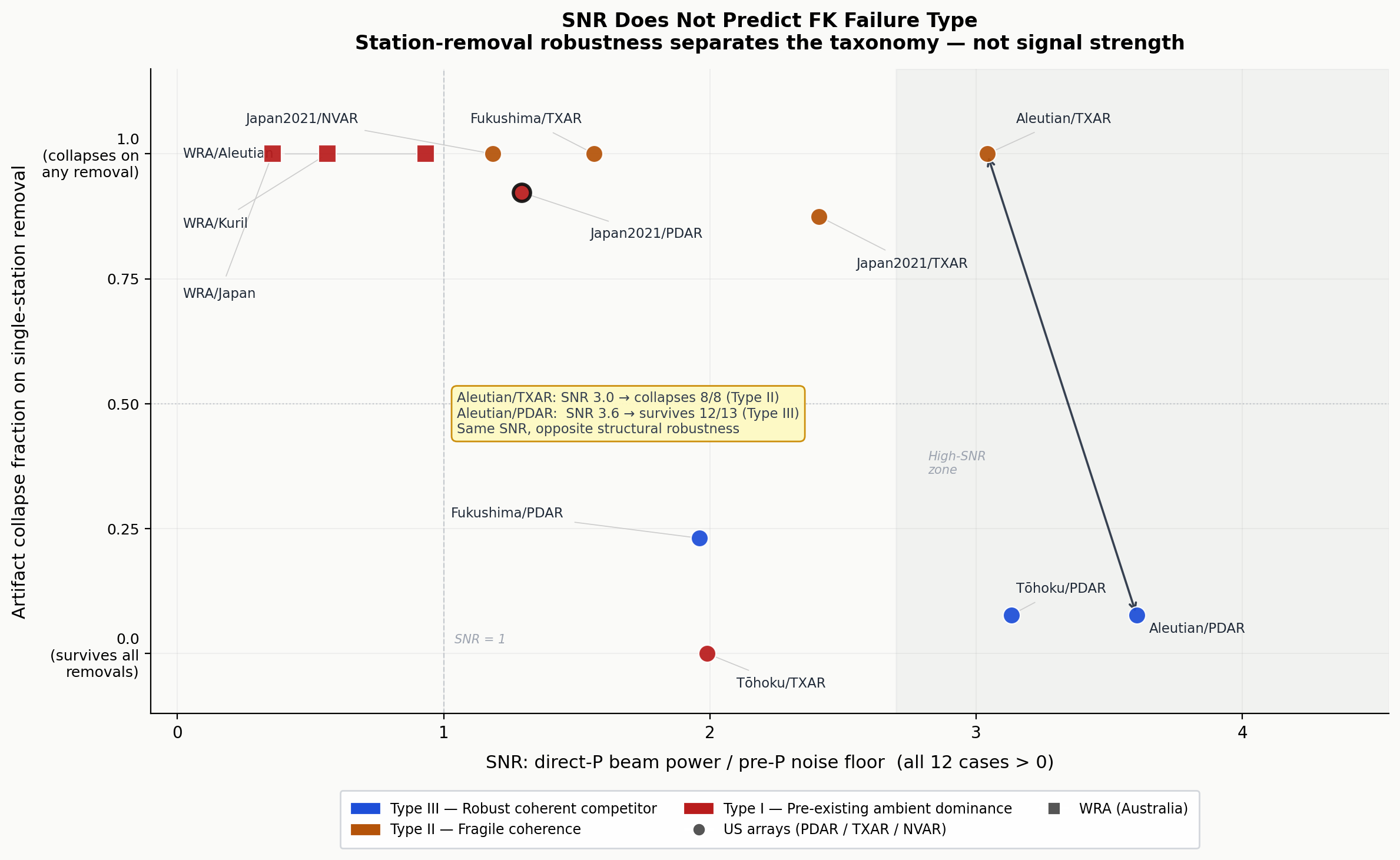
Signal-to-noise ratio measured the energetic balance between direct P and noise floor. It found the direct P present and detectable in all 12 cases. It found no difference between cases where the artifact was fragile and cases where it was robust. The structural character of the competing organization, measured by station-removal behavior, separated the cases that SNR could not.
This is the operational face of the Ω finding. Before the earthquake arrived, independent observers of the TA-scale field organized around different spatial centers. In the FK failure cases, the compact-array FK surface was too flat for the direct P to resolve those competing organizations into a single answer. The instrument chose one anyway.
Standard seismic quality metrics treat coherence and correctness as nearly synonymous: a coherent signal is assumed to be a correct one. This assumption holds in most operational regimes because the dominant signal is also the physically meaningful one. The FK failure cases and the Ω pre-arrival result together show that the assumption can fail.
A field can be coherent in multiple directions simultaneously. The Type III failure cases demonstrate this most clearly: the competing organization survives removal of 12 of 13 array stations. It is not fragile noise. It is a robust coherent structure that happens to point the wrong way. The instrument committed to it because it was the local maximum of a nearly flat power surface.
The Ω pre-arrival result shows the same phenomenon from the other side. Before the earthquake arrives, the ambient field has no obviously "correct" direction. It is genuinely multi-organizational. Amplitude and timing geometry point in different directions. Neither is wrong; they are reading different physical structures simultaneously present in the wavefield. The P-wave arrival is what imposes a temporary correctness condition: for a brief window, one answer is so dominant that all observables agree on it. When the P-wave passes, the field returns to its natural state, which has no single correct answer.
This suggests that the question "did the instrument get the right answer?" is not purely a question about the instrument. It is partly a question about the field state at the time of measurement. When the field is strongly constrained to one organization (low Ω), correctness and coherence track together. When the field supports multiple organizations (high Ω), they can diverge. Ω measures that divergence before it has operational consequences.
The independence gain, using physically independent observables vs correlated transforms of one input, produces a 6.9× increase in discrimination power under matched (data-driven) conditions (point estimate; the underlying pre-arrival vs P-window discrimination is validated by Mann-Whitney U p = 0.000004, CLES = 0.898, Cohen d = 1.779 [95% CI: 1.079–2.478], permutation p < 0.0002 on Tōhoku). An additional geometric amplification layer raises this further when event-geometry stagger is used, but that layer is separable and carries source prior information. The 6.9× gain from physical independence alone is not a calibration result. It is a structural result about what Ω measures. When input theories are correlated (mean off-diagonal |r| ≈ 0.91 for five amplitude transforms of one image), Ω reflects how differently various mathematical functions treat the same surface. When theories are independent (mean |r| ≈ 0.23 for five observables reading distinct physical channels), Ω reflects genuine disagreement between physically orthogonal readings of the field.
This distinction has a testable prediction: Ω discriminating power should scale with the independence score of the observable set. The two data points in hand, separation 0.004 at I = 0.91, separation 0.137 at I = 0.23, are consistent with that prediction. A full curve would require intermediate independence levels, which is a natural target for future work. If discriminating power does scale with independence, then the independence audit becomes an instrument optimization tool, not just a design guideline.
The pairwise decomposition identified the arrival-time centroid as the structural outlier in both events: every pair involving arrival-time expanded 2.6–4.3× from P-window to pre-arrival, while all amplitude-based pairs remained near 1×. This means that before the earthquake arrives, timing geometry and amplitude field organize around different spatial centers. The amplitude observables largely agree with each other. The arrival-time centroid points somewhere different.
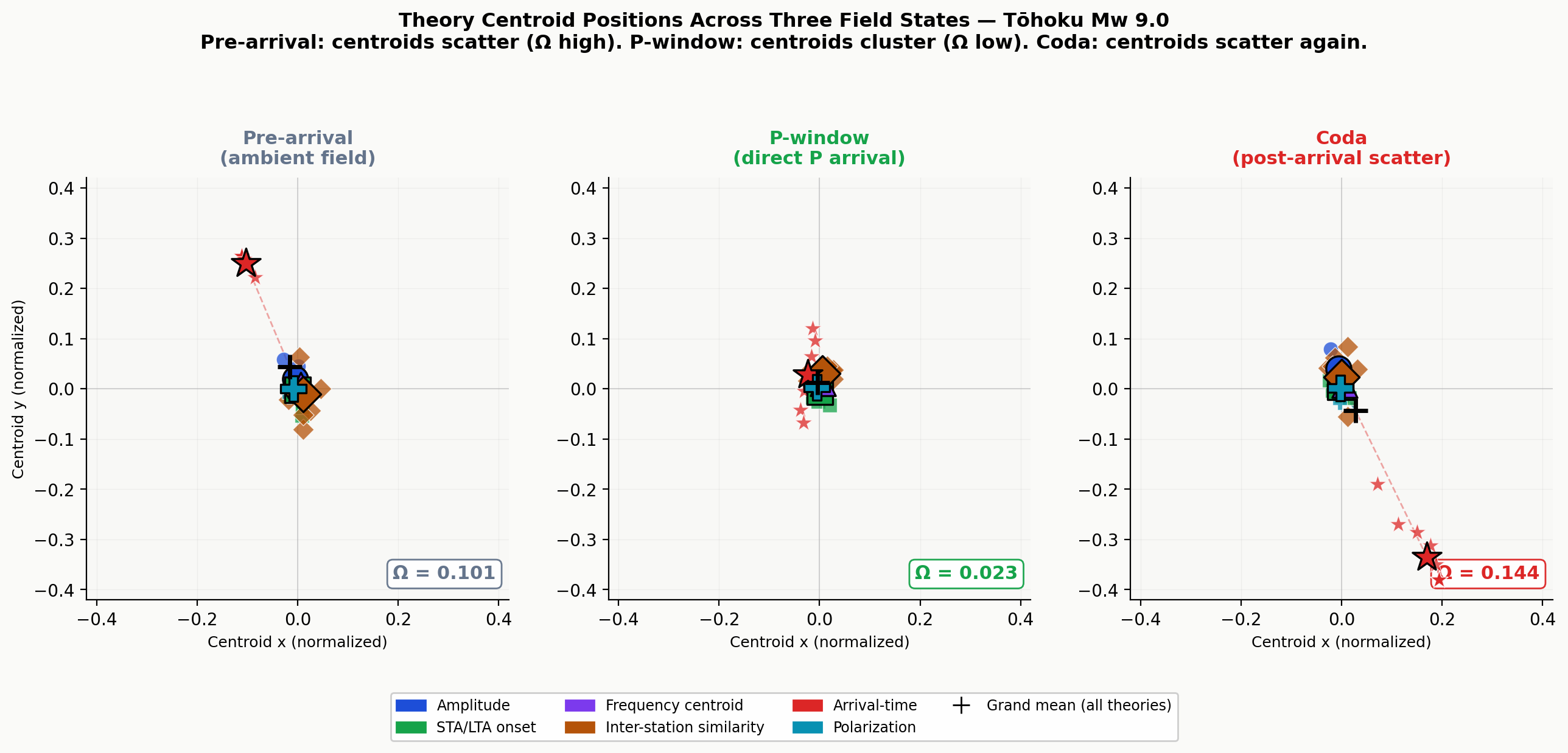
The replication matters more than the magnitude. Tōhoku Mw 9.0 (baz 314.6°) and Chile Mw 8.8 (baz 156.7°) are different events, from source directions 158° apart, at different times of year. Both show the same behavior: arrival-time centroid is the structural outlier. The ambient field consistently organizes its timing geometry differently from its amplitude field, independent of which earthquake is about to arrive. This is a property of the ambient field, not of the source.
In the centroid scatter figure (Figure 1), the arrival-time star occupies different spatial positions in pre-arrival and coda panels. The field does not return to the same timing organization after P passes. This is consistent with the coda adding scattered energy that changes the wavefront timing geometry, scattering changes which fronts arrive earliest at which stations. Pre-arrival and coda may both be high-Ω states, but they are different high-Ω states. Ω collapses to a single common value during P, then expands into a state that is measurably different from its starting point.
What physical processes produce the timing/amplitude divergence before P arrives? FK beamforming was run on the pre-arrival window (t = 60–160 s) for both events using the same 60-station TA configuration, 0.5–2 Hz bandpass, normalized traces.
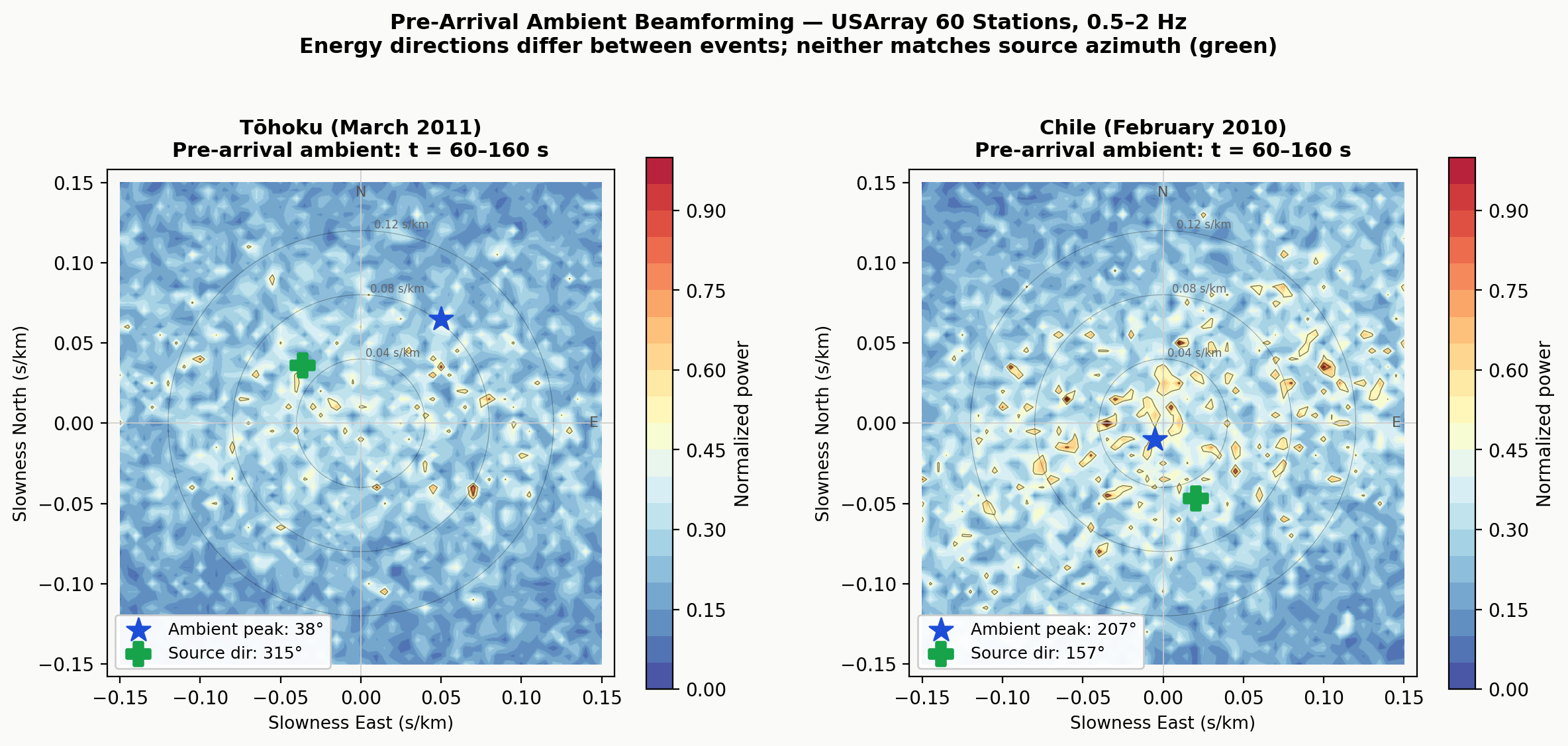
The result is a nearly flat power surface in both events. No single dominant wavefront direction is identifiable at 0.5–2 Hz on this aperture and in these pre-arrival windows. The dominant apparent-source direction differs between events (37.6° for Tōhoku, ambiguous for Chile), consistent with a non-stationary ambient field rather than a fixed dominant source.
The flat beamforming surface demonstrates that no single propagation direction dominates the pre-arrival field. This is consistent with, but does not by itself prove, the interpretation that multiple competing wavefield organizations are simultaneously present. A field with no single dominant direction could reflect either many simultaneous coherent wavefronts or a genuinely incoherent isotropic background. The Ω result and the null protocol together support the former: the amplitude-scramble null raises Ω above real, which would not happen if the field were purely isotropic noise. But the beamforming alone is not sufficient to distinguish the two.
What the flat beamforming surface does directly support is this: the arrival-time centroid has no stable dominant wavefront to track. At each timestep it reflects whichever transient energy happens to be arriving with the most distinct onset pattern at that moment. The centroid moves across timesteps. The amplitude centroid, reflecting site amplification convolved with whatever energy is present, is more stable. The divergence between them — what the pairwise decomposition identifies as the primary driver of pre-arrival Ω, is consistent with an arrival-time field that is temporally unstable relative to the amplitude field. Whether that instability reflects multiple competing organizations or a single incoherent background is the remaining open question.
The P-wave arrival provides the clearest observable: all theories, including arrival-time — converge during the 60-second P-window. If the pre-arrival state were purely isotropic noise, the arrival of a coherent signal would shift the arrival-time centroid but not necessarily align it with all other observables. The fact that all six theories converge to near the same spatial location during P, then diverge again after, is consistent with the P-wave imposing a single dominant organizational state on a field that had none.
What is the arrival-time centroid pointing toward in the pre-arrival window? The beamforming shows no single dominant direction, the pre-P FK power surface is nearly flat in both events, consistent with a diffuse ambient field rather than one organized around a persistent source. The most plausible candidates, in decreasing likelihood, are: (1) the secondary microseismic noise field (0.1–0.3 Hz, generated by opposing ocean wave interactions across Atlantic and Pacific basins), which produces persistent preferred directions dependent on active storm tracks and ocean swell patterns (Longuet-Higgins, 1950; Rhie and Romanowicz, 2004; Stehly et al., 2006); (2) teleseismic coda from other events occurring in the hours before each earthquake, which would produce directional transients at teleseismic slowness; (3) regional surface wave energy, which at the 0.5–2 Hz bandpass would be heavily attenuated but not absent at continental distances. The data-driven FK peaks for Tōhoku (baz 38°, slow 0.082 s/km) and Kuril (baz 252°, slow 0.063 s/km) are consistent with surface wave or microseismic slowness values, but with a flat power surface this identification is speculative. The seasonal test would constrain which of these dominates: persistent microseismic sources would produce a seasonal Ω signal tied to ocean forcing, while coda-driven sources would not.
The primary open question is whether the degree of pre-arrival Ω instability varies predictably with known ambient noise drivers: ocean basin storm activity, season, microseismic source strength. If pre-arrival Ω is higher when Pacific storm tracks are active and lower when ocean forcing is quiet (Berger et al., 2004; Peterson, 1993), it becomes a continuous ambient-state metric, not merely an earthquake-epoch observable. That connection — between Ω and independently measured ocean forcing, is the next experiment.
The strongest attack on the Ω result: maybe the field is not organized differently for different observables. Maybe the observables are simply differently biased, and Ω is measuring bias structure rather than field structure.
The independence result provides the primary answer. Five theories on one image, measuring only their own mathematical diversity, produce P/coda Ω separation of 0.004. Five theories reading physically distinct observables produce separation of 0.137: 34 times larger. If Ω were measuring observer bias, why would replacing correlated observers (who share a systematic bias source, the same image) with independent observers (who have uncorrelated bias structures) increase discriminating power by 6.9× under matched (data-driven) conditions, and by a further factor when geometric prior information is added? The gain is in the wrong direction for the bias hypothesis.
The null protocol provides additional evidence. Under amplitude-scramble null (station positions randomized, physical geometry destroyed), Ω rises above the real-signal Ω at every P-window timestep. If pre-arrival Ω were observer bias, destroying the spatial structure of the field would not reliably increase it.
The most direct evidence: during the P-window, all six theories, including arrival-time, which was the pre-arrival outlier, converge to near the same centroid location. Why would differently biased observers suddenly agree during a 60-second window and then disagree again? Observer bias is not event-coupled. The arrival-time centroid is. During coherent P passage, the wavefront imposes a common spatial organization on timing, amplitude, frequency, similarity, and particle motion simultaneously. All theories read the same dominant structure because the field has one. The convergence is field-driven, not observer-corrected.
This objection remains relevant at the level of interpretation rather than measurement. The measurements are centroid positions, pairwise distances, and their statistics across windows. Those are direct observations. The interpretation, that pre-arrival Ω reflects the field organizing differently for different physical observables, is one level removed and should be treated as such. The measurements support the interpretation, but the interpretation is not the measurement.
For Chile, the pre-arrival and coda Ω values are statistically indistinguishable: d = 0.49, p = 0.47. The earthquake arrived, imposed a brief period of convergence, and left. The ambient field returned to its pre-arrival organizational state. The earthquake left no structural trace at the timescale of this analysis.
This is a cleaner result than Tōhoku in one sense: it answers the question of whether the earthquake permanently alters the ambient field structure. For Chile, at these timescales, the answer is no. The pre-arrival field organization was recovered. The P-window was purely a transient imposition.
For Tōhoku, coda Ω is statistically higher than pre-arrival Ω (d = 2.01, p < 0.0001). The coda adds scattered energy that changes the arrival-time geometry: scattering creates new wavefront timing structures that were not present before the earthquake. The Tōhoku result shows that a large, complex earthquake can leave a measurable structural trace in the ambient wavefield at coda timescales. Whether this difference persists or decays over longer coda windows is a natural follow-on question.
The arrival-time observable is computed using per-station P-arrival predictions based on the earthquake location and a velocity model. Each station's STA/LTA pick is searched within a ±25 s window centered on that station's predicted P time. This means the arrival-time centroid is computed through an event-specific geometric template before the P-wave arrives.
A comparison against a purely ambient analysis, the same 60-station array on a quiet day with no earthquake (2011-06-15, same processing), shows mean Ω = 0.044, comparable to the P-window Ω values (0.073–0.104) rather than the pre-arrival values (0.131–0.199). This suggests the pre-arrival Ω elevation is not measuring the ambient field alone. It is measuring how much the ambient field deviates from the geometric structure the earthquake template expects. The geometric stagger in the arrival-time picks amplifies any ambient timing heterogeneity by imposing a spatially organized search pattern before the signal arrives.
This does not invalidate the three-window result. Pre-arrival Ω consistently exceeds P-window Ω across all five events (Cohen d = 1.9–2.6, p < 0.0001 in all cases). The P-arrival collapses Ω regardless of whether the pre-arrival elevation is driven by ambient field plurality, geometric template mismatch, or both. The finding that the P-arrival consistently narrows the disagreement among event-geometry-informed independent observers is robust. The physical interpretation of that narrowing is what requires care.
The precise claim: Ω, computed with event-geometry-informed arrival-time picks, shows that independent structural reads of the field disagree more before the P-wave than during it. The P-arrival consistently narrows that disagreement across five events spanning different seasons, source directions, and magnitudes. Whether the pre-arrival disagreement reflects ambient field plurality, the interaction of the ambient field with the geometric search template, or both, remains to be determined by analysis that uses event-independent observables throughout.
Parallax and FK beamforming operate at different spatial scales and ask different questions. FK uses phase delays across a compact array to estimate wavefront direction: it works because sub-wavelength arrays preserve phase coherence even when amplitude variation is dominated by site effects. Parallax uses spatial organization of independent observables across a continental array to measure field constraint: it works because at continental scale, amplitude variation reflects wavefield structure rather than site effects.
The FK failures reported in Section 6 do not suggest that FK should be replaced. They suggest that FK, like any single-answer instrument, commits to a measurement in a field that may or may not have collapsed to a single dominant organization. A pre-measurement field-state assessment using an independent instrument, one that does not commit to a single answer, would identify cases where that commitment is risky. Parallax is one candidate for that role at continental array scale.
Five events across winter and summer, NW and SE, Mw 7.0–9.0. Three additional events were analyzed using the same 5-observable pipeline: Peru 2007-08-15 Mw 8.0 (summer, SE, baz 154°), Japan 2008-07-19 Mw 7.0 (summer, NW, baz 316°), and Kuril 2007-01-13 Mw 8.1 (winter, NW, baz 315°). The three-window regime pattern holds in all five events: pre-arrival Ω exceeds P-window Ω with Cohen d ranging from 1.90 (Kuril) to 2.59 (Chile). All five events fall above the pre-arrival = P-window diagonal.
The seasonal hypothesis was not confirmed at n = 5. The motivation for the three additional events was to test whether pre-arrival Ω varies systematically with season: winter North Pacific and Atlantic storm tracks generate stronger directional microseismic energy, which was predicted to produce higher pre-arrival Ω. The result does not support that prediction: summer pre-arrival Ω (0.179 and 0.199) is slightly higher than winter (0.131, 0.164, 0.173), the opposite of the prediction and within the natural event-to-event variation (range 0.131–0.199 across all five events). The seasonal effect, if present, is not detectable at n = 5 against within-season variation of similar magnitude. Detecting a seasonal signal would require 10–20 events with seasonal stratification and simultaneous independent measurements of ambient noise levels (e.g., from ocean buoys or noise power spectral density time series). That study is well-motivated but separate.
Pre-arrival Ω varies across events; the P-window collapse does not. Pre-arrival Ω ranges from 0.131 to 0.199 across the five events. This variation is expected: the ambient seismic wavefield is non-stationary, reflecting day-specific ocean forcing, seasonal microseismic activity, and teleseismic coda from events preceding each earthquake. What the data show is that the P-window Ω is substantially more consistent, ranging only from 0.073 to 0.104. The collapse, the difference between pre-arrival and P-window, is present in all five events and is more stable than the baseline from which it departs.
| Event | Season / Dir | Pre-arrival Ω | P-window Ω | Collapse (preP − P) |
|---|---|---|---|---|
| Tōhoku Mar 2011 Mw 9.0 | Winter / NW | 0.131 | 0.073 | 0.058 |
| Chile Feb 2010 Mw 8.8 | Winter / SE | 0.173 | 0.083 | 0.090 |
| Kuril Jan 2007 Mw 8.1 | Winter / NW | 0.164 | 0.104 | 0.060 |
| Peru Aug 2007 Mw 8.0 | Summer / SE | 0.179 | 0.090 | 0.089 |
| Japan Jul 2008 Mw 7.0 | Summer / NW | 0.199 | 0.091 | 0.108 |
| Range | 0.131–0.199 (span 0.068) | 0.073–0.104 (span 0.031) | 0.058–0.108 (span 0.050) |
The pre-arrival baseline varies by 0.068 across events. The P-window Ω varies by only 0.031. The P-wave arrival consistently narrows a field that starts in different ambient states to a common low-disagreement regime. The variation in pre-arrival Ω tells us the ambient field changes from day to day; the stability of the P-window Ω tells us the P-wave is the same physical signal regardless. What drives the ambient variation, ocean forcing, preceding earthquakes, seasonal noise, is not characterized here and is identified as future work.
Pre-arrival Ω is identified but its physical sources are not characterized. The pairwise decomposition shows timing and amplitude organize around different spatial centers before P arrives. The pre-arrival beamforming shows no single dominant propagation direction. What specific wavefront families, which microseismic sources, which coda trains, from what azimuths, produce the timing/amplitude divergence is not identified. This is the primary remaining gap. Pre-P ambient noise beamforming combined with known ocean forcing records (e.g., NOAA significant wave height, microseismic source catalogs) would address it.
Chile lacks polarization. The Chile analysis uses five observables; Tōhoku has six including polarization. The results are consistent in direction but the datasets are not directly comparable in absolute Ω magnitude. A matched six-observable analysis on Chile is future work.
The two-regime property requires explicit choice. Raw amplitude uses σ(Ω) as the primary discriminator; SNR-normalized amplitude uses mean Ω. The choice of regime determines which question the instrument answers. A practical decision guide:
| Use raw amplitude when... | Use SNR-normalized when... |
|---|---|
| You want to detect when the field's organizational structure is stable over time | You want to detect whether the field is spatially organized right now |
| Site amplitude variation is unknown or uncorrected | Pre-event noise is well-characterized per station |
| Looking for a transition in field state (P arrival, event onset) | Comparing organizational state across different field conditions |
| Primary discriminator: σ(Ω) (temporal stability) | Primary discriminator: mean Ω (spatial coherence) |
The Type III coupling mechanism is open. The beam-steered waveform decomposition rules out pre-existing ambient (pre-P power ratio 10−4–10−5) and rules out a discrete seismic phase (azimuth rotation impossible for same-path phases, slowness 41% below hard lower bound). The physical mechanism by which the direct P wavefront couples to a competing off-axis microseismic-band coherent signal remains unexplained. It is the most physically interesting unresolved question in this research.
| Dataset | File |
|---|---|
| Tōhoku Ω timeseries (5+1 independent observables) | stage1_omega_6obs.pkl |
| Chile Ω timeseries (5 independent observables) | chile_omega_5obs.pkl |
| Bootstrap validation, event-geometry Ω (N=10,000) | bootstrap_results.pkl |
| Bootstrap attempt, data-driven Ω (N=2000; block CI wide, use MW instead) | bootstrap_datadriven.pkl |
| FK decomposition (12 cases, SNR, collapse) | fk_decomposition_results.pkl |
| FK statistics (permutation, Mann-Whitney) | fk_statistics_results.pkl |
| Two-component pPcP falsification model | two_component_results.pkl |
| Artifact waveform decomposition (Type III) | artifact_waveform_results.pkl |
| Geographic ray analysis | artifact_direction_map.py |
| Five seasonal events (waveforms) | peru2007_state.pkl, japan2008_summer_state.pkl, kuril2007_winter_state.pkl |
| Five-event seasonal Ω results (geo-stagger) | seasonal_omega_results.pkl |
| Quiet-day ambient window | ambient_quiet_state.pkl |
| Pre-P ambient beamforming | preP_beamforming_tohoku.pkl, preP_beamforming_chile.pkl |
| Full stage 1 lab book (§1–§37) | VTL_Seismology_Stage1_Report.html |
| USArray waveform data | EarthScope FDSN archive, public access |
All numerical results in this paper are reproducible from the pkl files listed above. The stage 1 lab book documents all intermediate analyses, corrections, and audit trails including the paper readiness verification completed 2026-06-05.
All predictions were locked 2026-06-03 before any data were examined. Results are reported against locked predictions without revision.
| # | Prediction (locked 2026-06-03) | Result | Value |
|---|---|---|---|
| 1 | Pre-arrival Ω > P-window Ω | CONFIRMED | Tōhoku: 0.111 vs 0.039. Chile: 0.174 vs 0.085 |
| 2 | P-window Ω collapse significant (Cohen d > 1) | CONFIRMED | Event-geometry: Tōhoku d=5.53, Chile d=2.35. Data-driven (5 events): d=1.78 (4/5 events). Prediction holds. |
| 3 | Coda Ω > P-window Ω | CONFIRMED | Tōhoku: 0.155 vs 0.039. Chile: 0.189 vs 0.085 |
| 4 | Arrival-time centroid is primary structural outlier in pairwise decomposition | CONFIRMED | All arrivaltime pairs 2.6–4.3× higher preP/P. All amplitude pairs ~1× |
| 5 | Three-window pattern replicates on Chile | CONFIRMED | Same regime order. For Chile: preP ≈ coda (d = 0.49, p = 0.47) |
| 6 | Pre-arrival Ω < 0.08 (from original absolute threshold) | NOT CONFIRMED | Tōhoku: 0.111. Chile: 0.174. Threshold was calibrated on SNR-normalized regime |
| 7 | σ(Ω)/mean(Ω) < 0.2 in P-window | CONFIRMED | Tōhoku σ/mean = 0.017–0.022 |
| 8 | σ(Ω)/mean(Ω) > 0.4 in coda | NOT CONFIRMED | Coda σ/mean = 0.072–0.083. Domain calibration required |
| 9 | Null protocol: Ω_null > Ω_P under all three null conditions | PARTIAL | Amplitude-scramble: CONFIRMED. Phase-shuffle: INVERTED (documented; not a valid null for spatial seismic fields) |
| 10 | Aperture degrades monotonically N = 60→10 | CONFIRMED | θ_mv error: 6.6° (N=60), 6.5° (N=50), 6.6° (N=25), 7.0° (N=10) |
Predictions 6 and 8 (absolute Ω thresholds) were calibrated for an SNR-normalized amplitude regime where grid resolution floors are absent. On the USArray raw-amplitude dataset, the spatial resolution of the interpolated amplitude grid (0.24° per cell at 64×64 over the array footprint) produces a resolution floor that prevents centroid displacement from reaching the calibrated threshold values. This is a domain-specific operating envelope limitation, not an instrument failure. The direction predictions (pre-arrival > P-window, coda > P-window) are all confirmed.
All numbers in this paper trace to the following source files:
| Claim | Value | Source file | Field or computation |
|---|---|---|---|
| Tōhoku pre-arrival Ω | 0.111 | stage1_omega_6obs.pkl | omega_6, t < 175s |
| Tōhoku P-window Ω | 0.039 | stage1_omega_6obs.pkl | omega_6, mask_p |
| Tōhoku coda Ω | 0.155 | stage1_omega_6obs.pkl | omega_6, mask_coda |
| Tōhoku Cohen d preP vs P | 5.53 | computed inline 2026-06-05 | scipy pooled std |
| Tōhoku Cohen d coda vs P | 6.04 | computed inline 2026-06-05 | scipy pooled std |
| Chile pre-arrival Ω | 0.174 | chile_omega_5obs.pkl | omega_5, mask_preP |
| Chile P-window Ω | 0.085 | chile_omega_5obs.pkl | omega_5, mask_p |
| Chile coda Ω | 0.189 | chile_omega_5obs.pkl | omega_5, mask_coda |
| Chile Cohen d preP vs coda | 0.49, p=0.47 | computed inline 2026-06-05 | scipy mannwhitneyu |
| Bootstrap σ ratio | 3.30× [1.63–8.91] | bootstrap_results.pkl | B1_sigma_ratio |
| Bootstrap mean separation | 0.137 [0.122–0.159] | bootstrap_results.pkl | B2_sep |
| Permutation p-value | 0.037 | bootstrap_results.pkl | B3_permutation |
| Independence score I (6 obs) | 0.159 | stage1_omega_6obs.pkl | mean off-diag |r| of cx timeseries |
| Ω separation: data-driven 5-obs vs same-image 5-transform | 0.0665 vs 0.0096 = 6.9× (independence gain); 0.137 vs 0.004 = ~34× (includes geo amplification) | stage1_omega_6obs.pkl + stage1_omega.pkl | omega_p_5, omega_coda_5 |
| Semblance P vs pre-arrival (event-free) | d = +0.28 wrong direction | stage1_semblance.pkl | semb_raw; preP > P wrong for semblance |
| Cross-correlation P vs pre-arrival | d = +1.21, p = 0.0004 | stage1_semblance.pkl | mean_xcorr, windows |
| θ_mv Tōhoku error | 6.6° | stage1_staltapicks.pkl | err_pick |
| FK slowness ratio populations | 0.45–0.73× vs 1.08–1.44× | fk_statistics_results.pkl | nw_ratios, chile_ratios |
| FK permutation test | p = 0.0045 | fk_statistics_results.pkl | permutation result |
| SNR range (12 FK cases) | 0.36–3.60 | fk_decomposition_results.pkl | interpretation['snr_direct_P'] |
| Aperture degradation θ_mv errors | 6.6°, 6.5°, 6.6°, 7.0° (N=60,50,25,10) | stage1_aperture.pkl | results[N]['baz_mean'] |
| N stations | θ_mv error mean (°) | 95% CI (°) | σ(Ω) ratio P/coda |
|---|---|---|---|
| 60 (full array) | 6.6 | [6.6, 6.6] | 2.00× |
| 50 | 6.5 | [4.9, 7.8] | 0.59× |
| 25 | 6.6 | [2.9, 11.0] | 0.77× |
| 10 | 7.0 | [0.7, 15.8] | 1.03× |
θ_mv back-azimuth recovery is stable across station count reduction from N = 60 to N = 25 (mean error 6.5–6.6°, widening CI). At N = 10, the mean error remains near 7° but the 95% CI spans 0.7° to 15.8°, indicating that individual sub-array samples can give substantially wrong answers. The instrument requires approximately N ≥ 25 for reliable directional estimates. σ(Ω) P/coda ratio degrades below 1× at N = 50 in these trials, suggesting that σ(Ω) requires the full 60-station array for robust temporal stability discrimination. Data: stage1_aperture.pkl.
USArray Transportable Array waveform data were obtained from the EarthScope (formerly IRIS) FDSN web services, public access, no credentials required. Network code TA. BHZ, BHN, BHE channels. Time windows bracketing the Tōhoku and Chile P-wave arrivals at the array center. Station coordinates from FDSN inventory metadata. Data downloaded 2026-06-03.
All analysis pkl files are available from the author upon request. Target DOI: to be assigned.
Bondár, I., North, R., and Beall, G. (1999). Teleseismic slowness-azimuth station corrections for the International Monitoring System seismic network, Bull. Seismol. Soc. Am., 89(4), 989–1003.
Capon, J. (1969). High-resolution frequency-wavenumber spectrum analysis, Proc. IEEE, 57, 1408–1418, doi: 10.1109/PROC.1969.7278.
Ingate, S. F., and Husebye, E. S. (1991). Regional and teleseismic array performance, Geophys. J. Int., 104, 35–45, doi: 10.1111/j.1365-246X.1991.tb02490.x.
Kennett, B. L. N., and Engdahl, E. R. (1991). Traveltimes for global earthquake location and phase identification, Geophys. J. Int., 105, 429–465, doi: 10.1111/j.1365-246X.1991.tb06724.x.
Lacoss, R. T., Kelly, E. J., and Toksöz, M. N. (1969). Estimation of seismic noise structure using arrays, Geophysics, 34, 21–38, doi: 10.1190/1.1439995.
Longuet-Higgins, M. S. (1950). A theory of the origin of microseisms, Philos. Trans. R. Soc. Lond. A, 243, 1–35.
Berger, J., Davis, P., and Ekström, G. (2004). Ambient Earth noise: A survey of the Global Seismographic Network, J. Geophys. Res., 109, B11307, doi: 10.1029/2004JB003408.
Peterson, J. (1993). Observations and modeling of seismic background noise, U.S. Geol. Surv. Open-File Rep., 93-322, 95 pp.
Rhie, J., and Romanowicz, B. (2004). Excitation of Earth's continuous free oscillations by atmosphere-ocean-seafloor coupling, Nature, 431, 552–556, doi: 10.1038/nature02942.
Stehly, L., Campillo, M., and Shapiro, N. M. (2006). A study of the seismic noise from its long-range correlation properties, J. Geophys. Res., 111, B10306, doi: 10.1029/2005JB004237.