Parallax Pathology
A Deterministic Structural Measurement Framework for H&E Histology
Evidence that Pathology can be framed as deviation in a structured geometric space.
ORCID: 0009-0008-9781-7995 · Copyright 2026
Abstract
Background. Current computational pathology systems classify tissue types with high accuracy but produce predictions without interpretable geometric explanation and require large labeled pathological datasets that do not exist for rare diseases. They ask what a tissue is. They do not ask how far a tissue has drifted from what it is supposed to be.
Instrument. Parallax Pathology is a deterministic, training-free structural measurement system for hematoxylin and eosin stained histology images. The system applies a 58-axis geometric and textural measurement framework to each image patch, computes a structural deviation scalar (Omega) representing distance from class-conditional structural norms, and produces axis-level explanations traceable to specific geometric properties. No trained parameters are used at any stage.
Findings. On the CRC-VAL-HE-7K benchmark (1,800 Macenko-normalized 224px patches, nine tissue classes), the system achieves 91.5% nine-class accuracy without any training, using only geometry, texture, and deterministic measurement. Deep learning foundation models trained on millions of labeled patches reach 95–99% on the same benchmark and that gap is real, acknowledged directly in this work, and not the point. The point is that a purely geometric, fully interpretable system gets that far at all, and produces something foundation models do not: an explanation grounded in the same structural properties a pathologist would read. Cross-dataset validation on three independent GTEx donors with PAXgene fixation confirms that structural centers emerge without labeled classes and that the measurement frame generalizes across preparation methods. A second cross-task validation on 920 EBHI-SEG enteroscope biopsy patches across six dysplasia grades achieves 84.3% correct-or-adjacent accuracy and ordinal Spearman r=0.716 (p=10⁻¹⁴⁵) with no training, confirming that the same 58-axis frame tracks continuous biological progression without modification. In a clinical outcome study on 180 TCGA-COAD patients (47 OS events, median follow-up 678 days), after Macenko stain normalization, eleven structural axes showed directionally consistent associations with both overall survival and disease-specific survival. A hybrid composite combining spatial openness, luminance-chromatic disagreement, and intra-tumor structural variability axes stratified patients with OS HR=1.687 [1.261–2.257] (p=0.0004) and DSS HR=1.872 [1.343–2.608] (p=0.0002), improving prediction beyond pathological stage. Signals concentrated in Stage III and IV disease. All survival findings are exploratory; External validation is required.
Positioning. Parallax Pathology is not a classifier competing with foundation models. It is a complementary measurement layer that does what trained systems do not: produce deterministic, interpretable, training-free structural measurements whose outputs are traceable to specific geometric and chemical properties of tissue. The intended architecture is hybrid, the 58-axis feature vector alongside foundation model embeddings, and structural deviation as an out-of-distribution signal alongside deep classifiers.
Keywords: computational pathology, structural measurement, deterministic analysis, anomaly detection, H&E histology, interpretable AI, structural deviation, survival prediction, spatial heterogeneity
1. Introduction
Computational pathology has achieved substantial accuracy in tissue classification and outcome prediction through deep learning. Foundation models trained on millions of labeled patches now approach the performance of specialist pathologists on standard classification tasks. Two structural limitations persist, however, and are unlikely to be resolved by scaling training data or model capacity.
The first is interpretability. A foundation model that classifies a patch as tumor cannot explain which geometric properties drove that prediction in terms a pathologist would recognize gland regularity, nuclear crowding, fiber alignment, and/or structural polarity. Gradient attribution methods attach post-hoc saliency maps to predictions, but these maps do not correspond to the geometric primitives a clinician reads. The explanation is derived from the prediction; it is not the prediction itself.
The second is data dependency. Every trained pathology model requires labeled pathological examples. For rare diseases where pathological datasets do not exist, the trained-model approach offers no path forward. The standard framing, learn what pathology looks like, is only as general as the training distribution.
Parallax Pathology inverts this framing. Rather than learning what pathology looks like, the system learns what normal structure looks like for each tissue type and measures how far observed tissue deviates from that norm. The pathology is not the input, it is the absence of normal form. A tissue type the system has never been exposed to will register as structurally distant from all known normal classes. A rare disease produces a meaningful signal without a single labeled pathological example.
The primary contributions of this work are:
- A deterministic, training-free 58-axis structural measurement system for H&E histology producing interpretable geometric and textural scalars per patch, all traceable to specific physical and chemical properties of tissue
- Validation on CRC-VAL-HE-7K demonstrating 91.5% nine-class linear accuracy without trained parameters, with biologically coherent structural separation across all tissue classes and an ablation confirming that geometry, texture, and microstructure encode genuinely complementary information
- Cross-dataset generalization on three independent GTEx donors with PAXgene fixation, establishing that structural centers emerge without labeled classes and characterizing which measurement axes are stable across preparation methods
- Cross-task progression detection on 920 EBHI-SEG enteroscope biopsy patches across six dysplasia grades, establishing that the same 58-axis frame tracks continuous biological progression with ordinal Spearman r=0.716 and 84.3% correct-or-adjacent accuracy, without modification or additional training
- Clinical outcome signal in 180 TCGA-COAD patients showing that spatial field organization, how structural states are distributed across tumor regions, associates with colorectal cancer survival after stain normalization, where mean structural deviation does not
All results are reproducible from published data files using documented, deterministic code. No GPU computation, model weights, or non-public data are required for any result in this paper.
2. The Instrument
2.1 Architecture
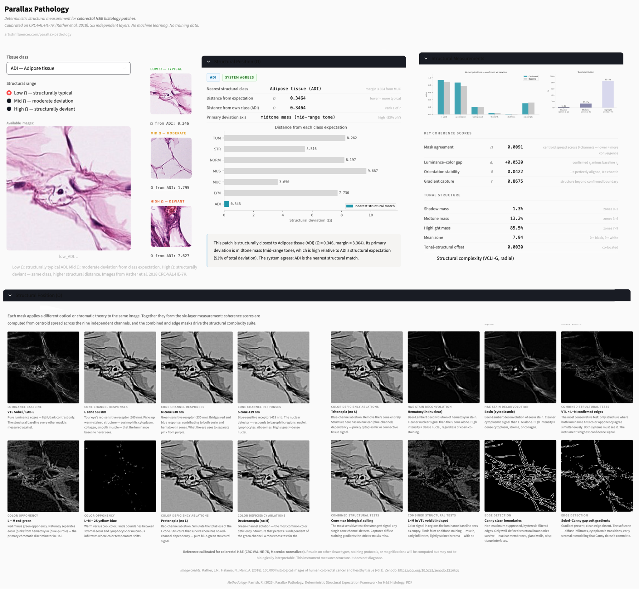
The system processes a single H&E image patch through nine sequential measurement layers, producing a flat vector of 58 scalar outputs. All computations are deterministic and stateless: the same image with the same configuration produces identical output on every run. All computations proceed on linear light after sRGB degamma is applied.
Layer 1: Kernel Primitives
Nine geometric scalars computed on both the confirmed edge field (the intersection of luminance and color opponency structural signals) and the raw luminance baseline. These primitives define the coordinate system in which all subsequent measurements are expressed: centroid position (Δx, Δy), void ratio (rᵥ), mass concentration (μ), spatial dispersion (SDI), packing density (ρᵣ), peripheral pull (X), orientation coherence (θ), and structural thickness (dₛ). Full mathematical specification is provided in Appendix A.
Layer 2: Sixteen Structural Masks and Coherence Scores
Sixteen independent structural theories are applied simultaneously to each image: the VTL baseline (Sobel edge detection on LAB L*), three LMS cone channels modeled using the Hunt-Pointer-Estévez D65 matrix, two opponent channels, three color deficiency ablations, two Beer-Lambert H&E deconvolution channels, three combined masks, and two Canny-derived masks. Four coherence scores are derived from mask comparison: Omega (mean pairwise centroid distance across masks), Gamma (boundary permissiveness), Delta-r (luminance-chromatic disagreement), and Beta (blind spot chromatic mass). The L+M-2S channel is systemically degenerate on standard brightfield H&E and is excluded from the structural expectation vector.
Layer 3: Structural Complexity
Complexity is measured across four components: centroid wander across scale (G1), void topology including count and aspect ratio (G2), contour curvature variance (G3), and orientation entropy slope over log-scale sigma values (G4). A Structural Coherence Index integrates these components.
Layers 4–5: Radial Compliance and Tonal Structure
Radial compliance measures how mass organizes relative to the frame center versus the patch's own center of gravity. Tonal structure maps LAB L* luminance into shadow, midtone, and highlight mass fractions, providing a preparation-sensitive but discriminating tonal profile.
Layer 6: Structural Expectation (Omega)
The structural expectation layer computes a class-conditional deviation scalar for each tissue class. For each class c, a reference encodes the mean feature vector and per-axis variance-inverse weights. The deviation scalar is computed as:
Low Omega indicates structural consistency with the reference class. High Omega indicates deviation, with axis-level decomposition identifying which geometric property is failing and in which direction. The system operates without knowing the tissue type label, it computes Omega against all reference classes and returns the nearest clinical class, the own-class distance when a label is available, the top driving axis, and the full per-class distance profile.
Layers 7–9: Texture and Microstructure Extensions
Layer 7 surfaces the gap mask (regions where Sobel gradient fires but Canny edge detection does not) as first-class metrics, characterizing soft gradient transitions associated with diffuse infiltrates and early stromal remodeling. Layer 8 computes Gray-Level Co-occurrence Matrix statistics on the LAB L* luminance channel at fine (cellular) and coarse (tissue) Gaussian blur scales. Layer 8b applies the same computation separately to the Beer-Lambert deconvolved hematoxylin and eosin channels, providing texture signals with direct chemical specificity. Layer 9 applies Difference of Gaussians blob detection to the hematoxylin channel to characterize nuclear density and size distribution across the patch.
2.2 The Frame-Memory Distinction
The most important architectural property of the system is the separation between the measurement frame and the reference memory. This distinction determines what the system can and cannot do, and why it generalizes across tissue types and preparation methods.
The frame is invariant. The 58 measurement axes define a fixed coordinate system for structural description. These axes are dataset-agnostic, non-learned, and interpretable. They define how structure is measured, not what structure should be. The frame does not change between colorectal and breast tissue, between formalin and PAXgene fixation, between a clinical slide and a whole-slide image.
The memory is inserted context. A reference memory is constructed from a corpus, the mean feature vector of that set, with per-axis variance-inverse weights reflecting how tightly each axis is constrained within that tissue type. The memory is dataset-specific, optional, replaceable, and not assumed to be universally correct. The system does not validate the memory; it reveals how observed data relates to it.
The deviation is the measurement. Omega measures distance from the inserted memory, not from an intrinsic notion of normality. A misaligned reference produces a correctly computed deviation field that reflects the distance between observed structure and the misaligned context. That deviation field is itself interpretable, and the misalignment is observable.
The practical implication is that the system requires no pathological examples to detect structural anomalies. Building a reference for a new tissue type requires only normal examples of that tissue. Normal tissue is almost always more available than labeled pathological datasets. This asymmetry is the primary access advantage for rare disease settings.
The frame-memory separation also implies a specific generalization architecture: a Library of Normals, in which the frame is held constant and references are built per-tissue-type, per-preparation-method, or per-institution. Each reference encodes the structural laws of its reference set. Deviation from those laws is the signal.
2.3 Relationship to Deep Learning Systems
On the standard colorectal histology benchmark (CRC-VAL-HE-7K, 1,800 patches, nine tissue classes), the system achieves 91.5% nine-class accuracy without any training. Foundation models trained on millions of labeled patches reach 95–99% on the same benchmark. That gap is real, acknowledged directly throughout this paper, and not the point. The point is that a purely geometric, fully interpretable system gets that far at all and produces something foundation models do not: a per-patch explanation grounded in the same structural properties a pathologist would read. No saliency map, no post-hoc attribution. The measurement is the explanation.
The gap exists because deep learning discovers features the designer did not specify. A convolutional network or vision transformer trained on millions of labeled patches learns representations capturing subtle, non-intuitive texture statistics, stain interactions, and spatial frequencies that no hand-designed primitive encodes. This is a genuine advantage of learned representations.
Parallax Pathology does not attempt to close this gap. It answers a different question. A foundation model answers: what is this tissue? It produces a confident categorical prediction, typically without explanation of which image properties drove the confidence. This system answers: how far is this tissue from what tissue of this type is supposed to do structurally, and which geometric axis is failing? It produces a continuous deviation scalar with axis-level explanation, without any training on pathological examples.
Three capabilities follow from asking the different question:
- Out-of-distribution detection. A deep classifier trained on colorectal tissue has a training distribution. An unseen tissue type will be assigned to the nearest training class with high confidence; the model has no mechanism for identifying that the geometry does not fit any known structural regime. High Omega on an unseen tissue type is the correct output, not a misclassification.
- Low-data and rare disease settings. Building a structural expectation reference requires only labeled normal tissue. Building a deep learning classifier requires large labeled pathological datasets that frequently do not exist for rare conditions.
- Intrinsic interpretability. The explanations produced by this system, such as delta-r is elevated, meaning luminance edges exist where color channels do not confirm them, are built into the measurement itself. They are not derived from the prediction; they are the prediction. This distinction matters in contexts where the explanation is as important as the result.
The intended relationship is hybrid, not competitive. The 58-axis structural feature vector is a structured, biologically interpretable representation that can be concatenated with any foundation model embedding. The combination carries both high-accuracy learned features and geometrically interpretable structural measurements. Omega used as an out-of-distribution signal alongside a deep classifier produces a system that is both accurate and capable of flagging patches outside the training distribution.
3. Tissue Classification Validation
3.1 Dataset and Setup
CRC-VAL-HE-7K (Kather, Halama and Marx, 2018) consists of 100,000 histological images of human colorectal cancer and healthy tissue. This study uses the 1,800-image stratified validation subset: 200 patches per class across nine tissue types at 224×224 pixels and 0.5 microns per pixel, Macenko-normalized to minimize stain variability. Classes include seven clinical types, tumor epithelium (TUM), cancer-associated stroma (STR), normal colon mucosa (NORM), lymphocytes (LYM), mucus (MUC), smooth muscle (MUS), and adipose tissue (ADI) - and two non-clinical types, debris (DEB) and background (BACK).
The structural expectation reference was built from the same 1,800-patch corpus. Per-class mean and variance were computed over the six-axis structural vector for all nine classes. Accuracy was evaluated using Linear Discriminant Analysis with five-fold stratified cross-validation (random_state=42), identical methodology across all reported comparisons.
3.2 System Performance
The full 58-axis system achieves 91.5% nine-class linear accuracy on CRC-VAL-HE-7K without any trained parameters. Every tissue class improves over the six-axis geometry-only baseline. The confusion pattern is biologically interpretable rather than random: errors concentrate at structurally adjacent class boundaries, consistent with the locations where pathologists exercise judgment.
| Class | Accuracy | Primary confusion | Biological reading | Dominant structural axis |
|---|---|---|---|---|
| ADI | 99% | — | Geometrically isolated; vacuolar architecture | k_rv, highlight_mass |
| BACK | 100% | — | Background glass; perfectly separated | highlight_mass alone |
| DEB | 93% | STR, TUM | Cellular fragments; mixed signal | delta_r, gamma |
| LYM | 96.5% | — | Isotropic nuclear packing; tightest theta constraint | theta (weight 6,388) |
| MUC | 97.5% | NORM | Void-dominant; high k_rv defines the class | k_rv, gamma |
| MUS | 81.5% | STR (33) | Highest theta class; parallel fiber organization | theta, delta_r |
| NORM | 95% | TUM (6) | Organized glandular crypts; moderate complexity | theta, highlight_mass |
| STR | 74.5% | MUS (28) | Structurally adjacent to MUS at 224px | delta_r, H/E texture |
| TUM | 86.5% | NORM (16) | Dense epithelial sheets; high midtone mass | midtone_mass, theta |
Visual example of ADI (Adipose)
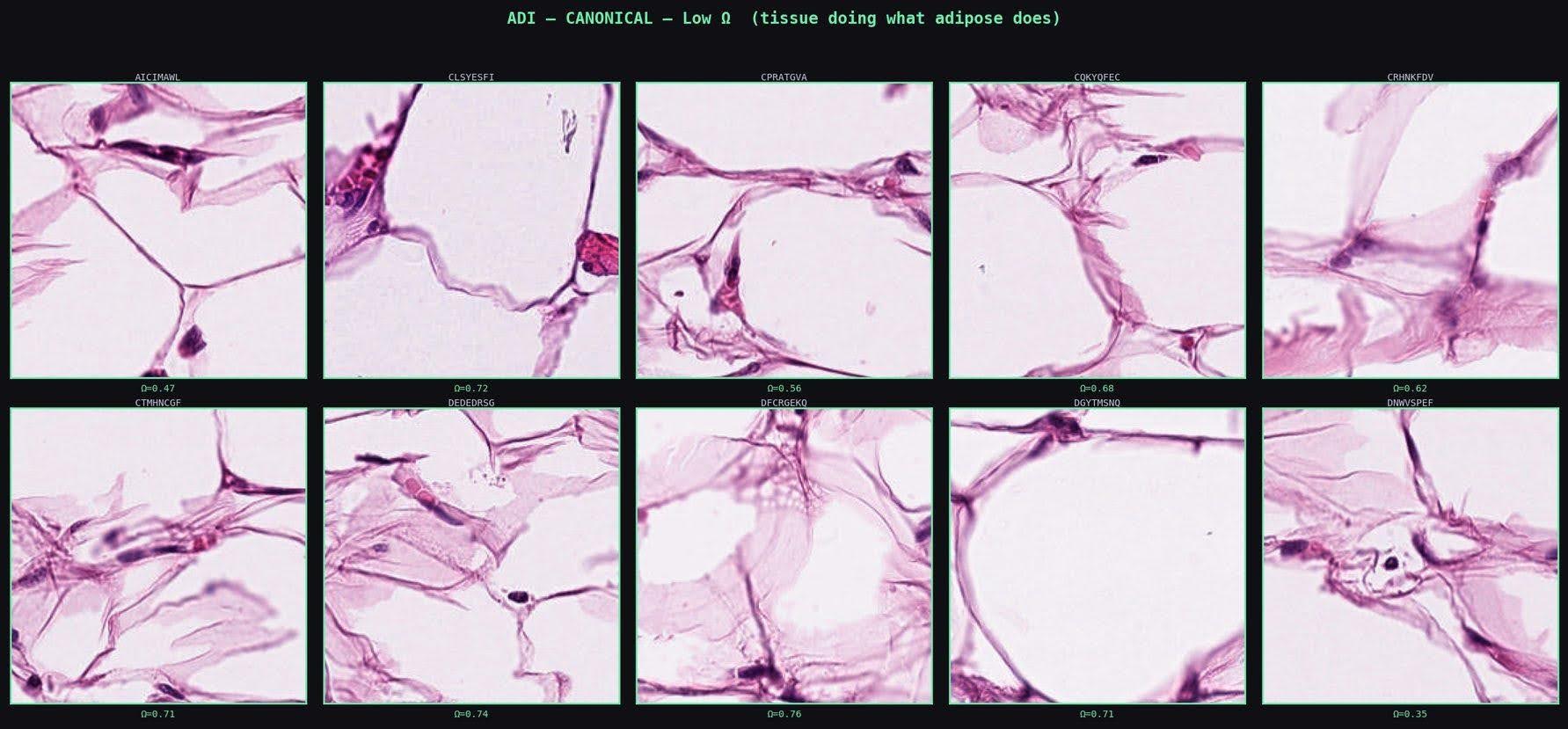
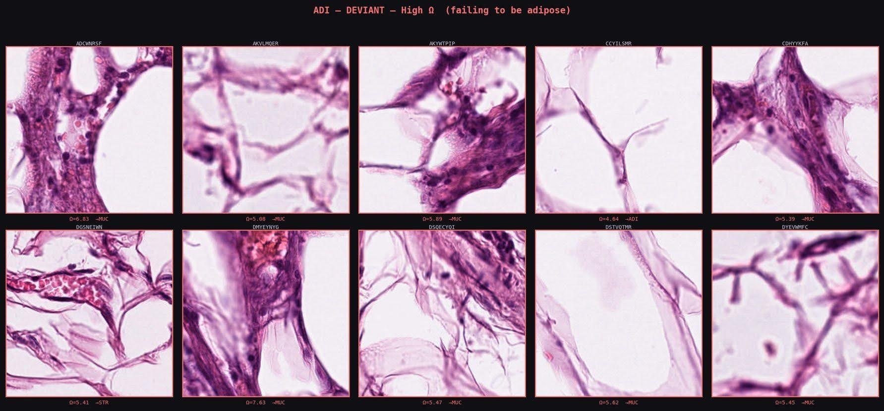
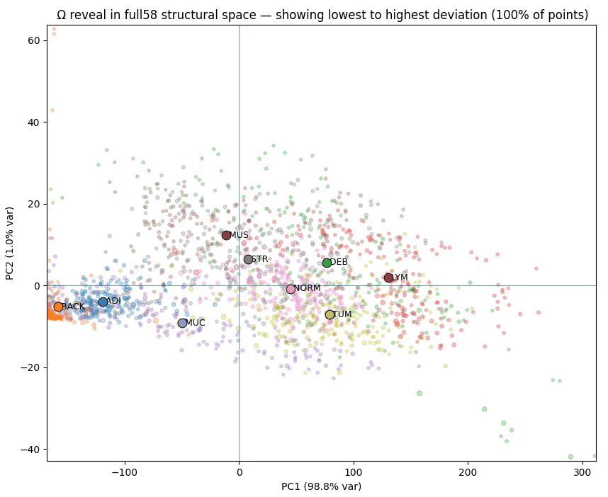
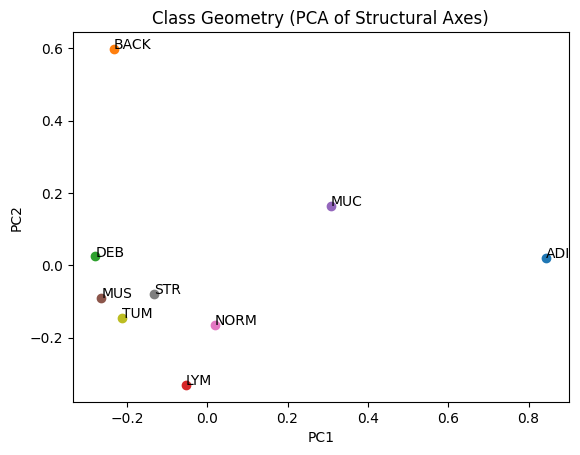
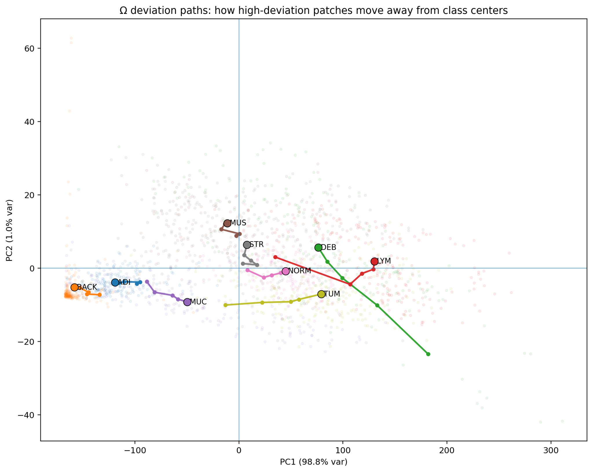
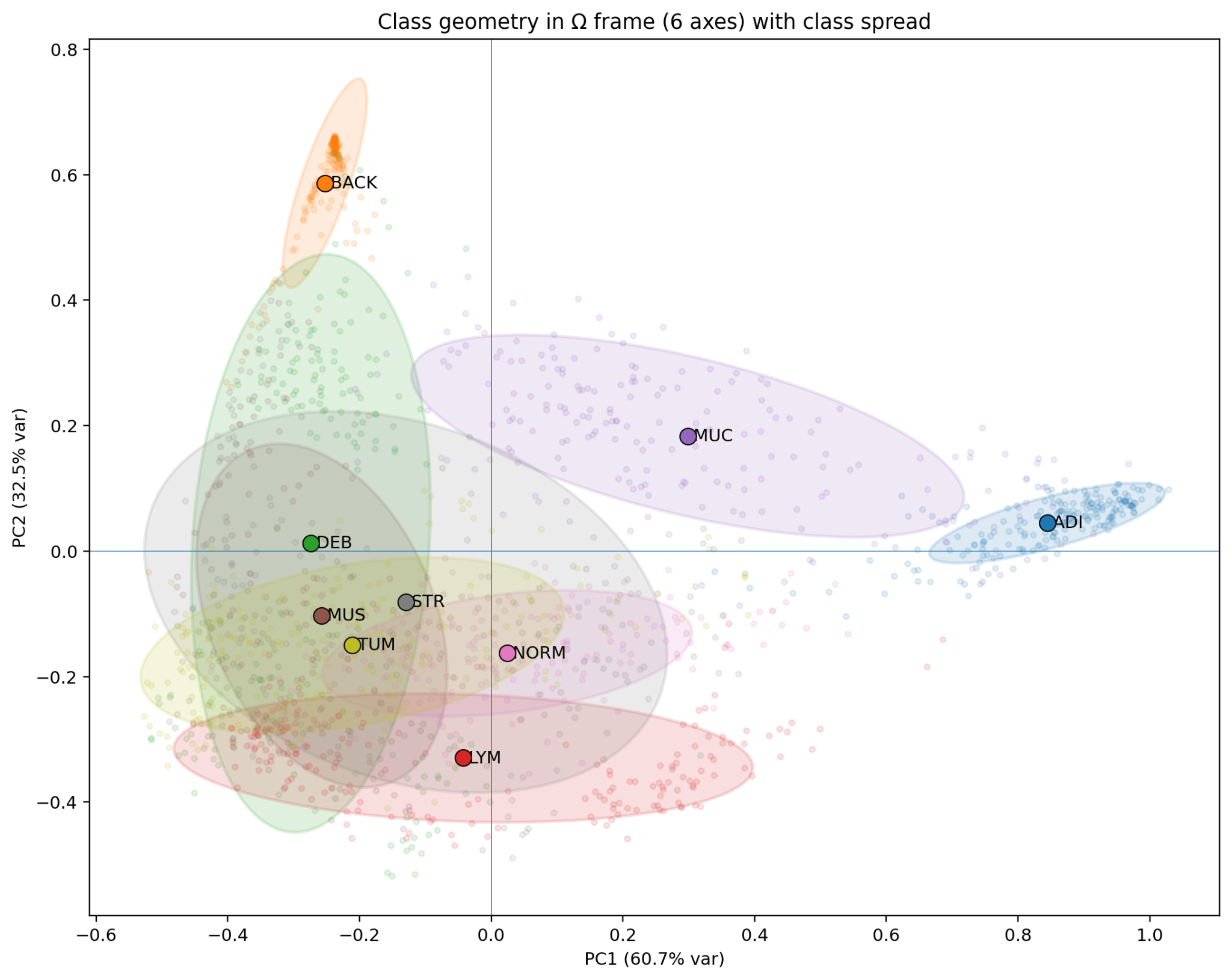
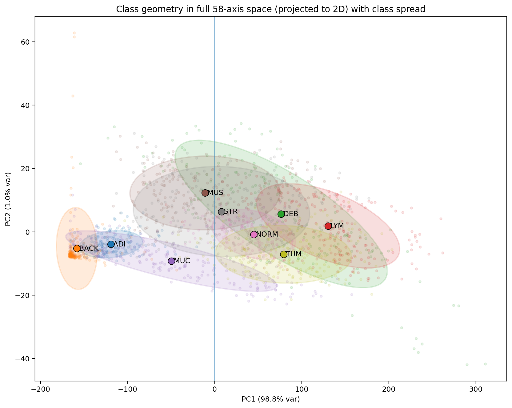
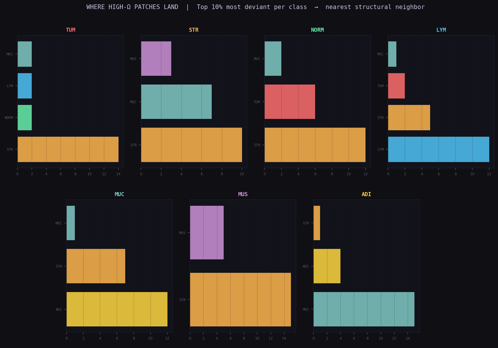
Projections of a defined structural coordinate system. These figures move from a simplified overview of class structure to the full representation used by the system. We begin with class centroids to show where each tissue type sits on average, then introduce spread and covariance to reveal how wide and directional each class is. From there, the Ω frame isolates the core structural axes, showing what macro-geometry alone can separate. Finally, the full 58-axis projection demonstrates how additional texture and microstructure features expand that space, increasing separation while preserving the underlying relationships between classes.
3.3 The Emergence Result
An ablation study evaluated each feature layer independently using identical LDA five-fold CV methodology. The key finding is the emergence gap: the best standalone layer (the six-axis geometry-only Omega vector at 75.2%) is 16.3 percentage points below the full system at 91.5%. No individual layer approaches combined performance.
| Layer | Axes (n) | Accuracy | Strongest contribution |
|---|---|---|---|
| Omega6 geometry only | 6 | 75.2% | Baseline; orientation coherence, void structure, tonal axes |
| L* GLCM luminance texture | 8 | 68.6% | tex_homogeneity_fine (+5.1pp in greedy selection) |
| H/E channel GLCM texture | 6 | 66.8% | Highest standalone STR accuracy (50.5%) |
| Gap mask and blob detection | 5 | 60.2% | gap_rv, blob_count, blob_size_cv |
| Full system (all layers) | 58 | 91.5% | Emergence from complementary layer combination |
The cancer-associated stroma class (STR) illustrates the emergence most clearly. Standalone STR accuracy ranges from 35.5% (gap mask alone) to 50.5% (H/E channel texture alone). The full system achieves 74.5%, a 24-point jump from the best standalone layer that cannot be attributed to any single addition. The covariance structure of the full feature set, how H/E texture, orientation coherence, and nuclear density co-vary across patches, is what the LDA exploits.
The greedy forward search found no additional accuracy gain beyond 58 axes. Every remaining unused numeric column in the feature space either added negligible signal or slightly reduced accuracy. This represents the ceiling of what a single 224px H&E patch can express deterministically at 0.5 microns per pixel under the current framework. A note on scale: the 224px ceiling is a property of the CRC-VAL-HE-7K benchmark, which is natively 224px and cannot be meaningfully upsampled. The framework itself is not limited to this resolution. The clinical survival analysis in Section 5 processes tiles at 512px natively, and the measurement pipeline has been applied at 448px. Larger field-of-view analysis, capturing gland spacing, tumor budding, and architectural grade, requires tiling from source whole-slide images, which is active development rather than a fundamental constraint of the measurement system.
3.4 TUM Deviant Analysis: Two Failure Modes
The tumor epithelium class produced the most clinically significant finding from the tissue classification study. High-Omega TUM patches drift predominantly toward STR, but metric analysis reveals two geometrically distinct failure modes within that drift.
Failure Mode 1 Density Loss. Six deviant patches show highlight_mass jumping from the canonical mean of 0.229 to 0.54–0.61, with gamma spiking to 0.60–0.67. The tumor field opens; cellular density gives way to optically permissive space. The geometric signature corresponds to mucinous differentiation, intratumoral necrosis, or poorly cohesive growth patterns.
Failure Mode 2: Directional Acquisition. Two deviant patches show theta jumping to 0.12–0.13, nearly five times the canonical TUM mean of 0.024. These patches have acquired directional structure that tumor epithelium normally lacks. The geometric signature corresponds to desmoplastic reaction: host stromal fibrosis within the tumor field. Both phenomena were detected from structural geometry alone, without training on either.
These two failure modes are geometrically orthogonal: one involves the tumor field losing density along the void and boundary axes; the other involves the tumor field acquiring coherent directionality along the orientation axis. Their biological readings, mucinous/necrotic differentiation and desmoplastic stromal reaction, are clinically recognized phenomena that this system detected from first principles.
3.5 Structural Drift Patterns
Across all clinical classes, high-Omega patches drift toward structurally adjacent classes in biologically coherent directions. Smooth muscle patches drifting toward stroma are losing fiber organization, theta declines as fascicles cut at angle and directional commitment collapses. Adipose patches drifting toward mucus show vacuolar architecture breaking down as spaces fill and cell walls distort. Tumor patches drifting toward normal mucosa reflect borderline architectural states at the adenocarcinoma boundary, the precise location where pathologist agreement is lowest.
These drift patterns are not artifacts of the classifier. They are properties of the geometric measurement space: tissues that are failing to maintain their structural identity move toward the class whose geometry they are acquiring. The Omega score quantifies the magnitude of that movement; the axis decomposition identifies the geometric mechanism.
4. Cross-Task Validation: Structural Progression Detection
4.1 Setup
The tissue classification validation established that the 58-axis system occupies a linearly separable structural space across geometrically distinct tissue types. A second independent validation tests whether the same instrument, without modification, can track a continuous biological progression, one where adjacent classes overlap by design and the task is not categorical identification but ordinal measurement of structural disorganization.
4.1 Dataset and Task
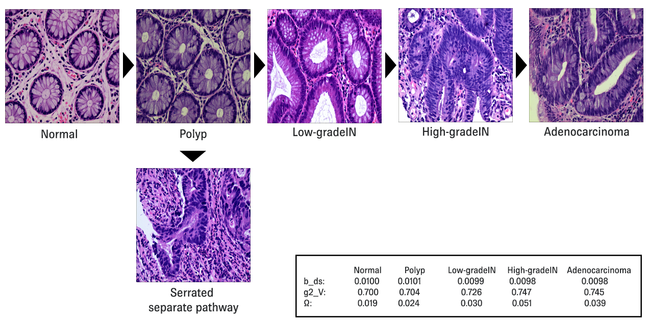
The EBHI-SEG dataset (Enteroscope Biopsy Histopathological H&E Image Dataset for Segmentation Tasks) provides 920 patches across six dysplasia grades at 224px: Normal, Polyp, Serrated Adenoma, Low-grade Intraepithelial Neoplasia, High-grade Intraepithelial Neoplasia, and Adenocarcinoma. Unlike the nine CRC-VAL tissue classes, which represent geometrically distinct tissue types, these six classes represent a continuous biological progression in the same tissue. Adjacent grades overlap structurally by nature. The task is not classification in the usual sense. It is whether a structural measurement instrument can track disorganization as a continuous variable.
To pressure test the initial study, no Macenko normalization was applied. The structural expectation reference was built from the EBHI data itself using the same Reference Builder workflow as CRC-VAL. No grade-labeled examples were used at any stage of measurement. The 58-axis feature set was transferred from CRC-VAL without modification.
4.2 Accuracy and Ordinal Performance
Six-class LDA with five-fold stratified cross-validation achieves 68.1% macro-average accuracy. Chance level for six classes is 16.7%; the system performs 51.4 percentage points above chance.
The headline accuracy number requires context. Six-class dysplasia grading on biologically continuous adjacent classes is structurally harder than tissue type classification. Pathologists themselves show inter-observer variability at the Low-grade/High-grade and High-grade/Adenocarcinoma boundaries. The confusion matrix reflects this: 86% of Adenocarcinoma errors land in High-gradeIN or Low-gradeIN, not in Normal or Polyp. Errors are grade-adjacent, not random.
The more informative metric is ordinal: 84.3% of all predictions are correct or within one adjacent grade step. The ordinal Spearman correlation between predicted grade rank and actual grade rank is 0.716 (p=10⁻¹⁴⁵). Ridge regression treating grade as a continuous outcome explains 41% of grade variance. A system producing random grade assignments would show Spearman r near zero and correct-or-adjacent accuracy near 50% for six classes. The instrument is tracking a coherent biological ordering.
| Metric | Value |
|---|---|
| Six-class LDA accuracy (macro) | 68.1% |
| Correct + adjacent grade | 84.3% |
| Ordinal Spearman r | 0.716 |
| Ridge regression R² | 0.41 |
| Kruskal-Wallis (g4_s8) | H=220 |
| Spearman axes p<0.001 | 11 |
| Training examples required | 0 |
| Dataset | n=920 |
4.3 Eleven Structural Axes Track Dysplasia Grade
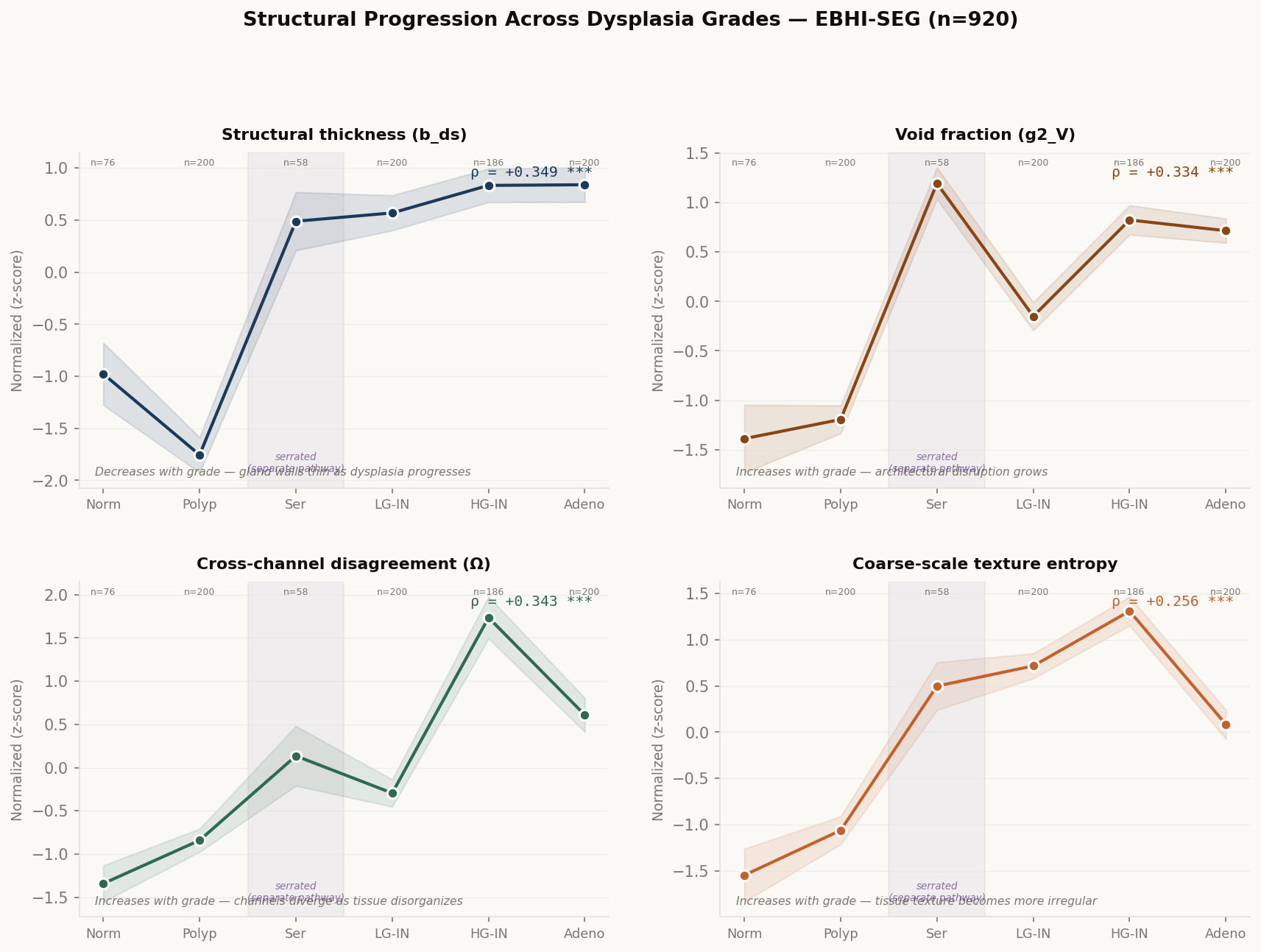
Independent of classification accuracy, eleven structural axes show statistically significant monotonic correlation with dysplasia grade. The top axes reach p<10⁻²⁰ or better. The strongest single axis is g4_s8 (orientation entropy at tissue scale): Kruskal-Wallis H=220, p=10⁻⁴⁵.
The biological reading is coherent across axes. Dysplastic tissue loses gland wall thickness (b_ds decreases, ρ=−0.349), develops more void space as glandular architecture disrupts (g2_V increases, ρ=+0.334), loses multi-scale orientation hierarchy as epithelial polarity degrades (g4_slope decreases, ρ=−0.304), and shows increasing disagreement between luminance and color structural channels as nuclear crowding progresses (omega increases, ρ=+0.343). These are independent measures of the same underlying process: progressive loss of organized glandular architecture.
| Axis | ρ | p-value | Biological reading |
|---|---|---|---|
| g4_s8, orientation entropy σ=8 | -0.299 | 1.84e-20 | Tissue-scale directional coherence lost as dysplasia progresses. Strongest Kruskal-Wallis: H=220, p=10⁻⁴⁵ |
| gap_rv, gap mask void ratio | +0.257 | 2.33e-15 | Soft gradient regions increase. More diffuse boundaries, less crisp gland wall definition |
| g2_V, void fraction | +0.334 | 2.38e-25 | Architectural void space grows. Glandular lumens dilate and disrupt |
| omega, mask channel agreement | +0.343 | 8.52e-27 | Cross-channel structural disagreement increases. Luminance and color channels diverge |
| b_ds, structural thickness | -0.349 | 1.08e-27 | Gland wall thickness decreases. Epithelial structures thin and lose definition |
| g4_slope, entropy slope | -0.304 | 4.58e-21 | Loss of multi-scale organizational hierarchy. Ordered tissue has steep entropy drop; dysplastic tissue does not |
| g1_len, centroid wander | +0.289 | 4.18e-19 | Mass center shifts more across blur scales. Structural heterogeneity increases |
| tex_entropy_coarse, texture | +0.257 | 2.77e-15 | Tissue-level texture becomes more irregular. Coarse pattern regularity breaks down |
4.4 The Serrated Pathway: A Structural Finding, Not an Error
The Serrated Adenoma class shows apparent non-monotonicity on several axes relative to its nominal grade position. This is not a system failure. Serrated adenoma follows a separate molecular pathway from conventional adenomas, BRAF mutation rather than KRAS, and has a distinctive saw-toothed glandular architecture that produces geometrically distinct structural signatures. On void fraction (g2_V), Serrated patches score 0.755, higher than both Polyp (0.704) and Low-gradeIN (0.726). The system is correctly measuring that serrated architecture is geometrically distinct from conventional low-grade dysplasia.
Evaluated on the conventional pathway alone (Normal, Polyp, LG-IN, HG-IN, Adenocarcinoma; n=662), correct-plus-adjacent accuracy reaches 88.2% and ordinal Spearman r=0.72. The serrated non-monotonicity disappears because serrated adenoma was never on the conventional progression scale to begin with. A system that forced Serrated perfectly onto the linear grade axis would be imposing a biological assumption the data does not support. The non-monotonicity is a finding, not a failure.
4.5 Instrument Generalization
The 58-axis feature set was selected on CRC-VAL tissue type classification. It was not tuned, re-selected, or adapted for the EBHI task. The grade progression signal is present in a feature set designed for a different task on a different dataset. This demonstrates that the structural axes capture genuine tissue organization properties that transfer across contexts rather than dataset-specific statistical patterns.
Together with the CRC-VAL classification results and the GTEx cross-dataset generalization, this validation establishes that the instrument operates across task types: tissue type classification, preparation method generalization, and now continuous biological progression detection. The measurement frame is the same in all three cases. The reference memory and the question being asked change. The instrument does not.
5. Cross-Dataset Generalization
5.1 Setup
Three independent GTEx whole-slide images were analyzed to test whether structural centers emerge without labeled classes and whether the measurement frame generalizes across preparation methods. All three donors used PAXgene tissue fixation, a different preparation chemistry from the formalin-fixed CRC-VAL-HE-7K dataset.
The three slides represent two mucosal donors (GTEX-S7SF-1926, colon transverse, female 20–29; GTEX-U4B1-1126, colon transverse, male 40–49) and one muscularis donor (GTEX-11ZTS-1526, colon sigmoid, female 60–69). Five hundred patches were extracted from each slide. No cross-normalization, stain normalization, or label alignment was applied. The frame is fixed across all three datasets; the reference memory is dataset-specific.
5.2 Structural Centers Emerge Without Labels
Each dataset was treated as an independent structural system. A donor-specific structural expectation reference was constructed from the 500 patches of that slide. Omega was then computed for every patch against its own reference.
All three datasets exhibit the same distributional structure observed in the CRC-VAL results: a concentrated central mass with an extended upper tail. Mean within-set Omega (2.09–2.26) is consistent with the CRC-VAL NORM mean of 2.16. This convergence across three independent donors, a different fixation method, and two different tissue compartments suggests the Omega scale is not arbitrary, but a similar central tendency emerges from similar internal structural coherence regardless of preparation context.
The void ratio (k_rv) correctly tracks tissue type across all three donors without any label input: muscularis (0.687) is denser than mucosa (0.779, 0.905), consistent with the biological difference between compact muscle fiber and open glandular architecture. This geometric property is stable across preparation methods.
5.3 Stable vs. Preparation-Sensitive Axes
Axis-specific analysis comparing high-Omega to low-Omega patches within each dataset reveals a consistent partition between stable and preparation-sensitive measurement axes.
Stable axes (k_rv, theta). Orientation coherence and void ratio carry consistent biological signal across all four datasets regardless of fixation method. In the muscularis donor, high-Omega patches drift toward open, high-void structure, away from the dense fiber organization that defines muscularis tissue. In both mucosal donors, theta is elevated in high-Omega patches, indicating directional acquisition as the shared mucosal failure mode.
Preparation-sensitive axes (delta_r, highlight_mass, midtone_mass). Luminance-chromatic disagreement (delta_r) inverts its role in the deviation field between fixation methods. In formalin-fixed CRC-VAL tissue, deviant patches show higher delta_r, luminance edges exist where color channels no longer confirm them. In PAXgene-fixed GTEx tissue, deviant patches show lower delta_r, structural failure involves a collapse toward channel uniformity rather than luminance-color dissociation. This inversion reflects preparation chemistry differences in how fixation methods interact with chromophore accessibility, not a measurement failure.
The practical implication for cross-site use: when building a structural expectation reference for a new preparation method, the stable axes (k_rv, theta) provide robust cross-site comparison. The full 58-axis system maximizes within-site accuracy but requires preparation-matched reference construction for texture axes to produce valid Omega deviation scores.
The frame is universal. The memory is not and should not be.
6. Clinical Signal: TCGA-COAD Survival Analysis
6.1 Dataset and Methods
Pre-tiled 512x512 pixel JPEG patches at 0.5 microns per pixel were sourced from Zenodo record 3784345 (Kather et al., 2020), tumor-only regions from TCGA-COAD whole-slide images. Clinical survival data were obtained from the TCGA Pan-Cancer Clinical Data Resource (Liu et al., 2018). After merging on patient barcode and filtering for complete overall survival and pathological stage data, the analysis cohort comprised 180 patients.
| Parameter | Value |
|---|---|
| Total patients | 180 |
| OS events (deaths) | 47 (26.1%) |
| DSS events | 36 (20.0%) |
| PFI events | 58 (32.2%) |
| Median follow-up (OS) | 678 days (1.9 years) |
| Stage distribution | I: 31 (17.2%) / II: 68 (37.8%) / III: 50 (27.8%) / IV: 31 (17.2%) |
| Tiles processed | 9,010 (approximately 50 per patient) |
| Stain normalization | Macenko (pure numpy, reference: TCGA-AA-3710) |
| Structural features | 58-axis Parallax Pathology, deterministic |
All tiles were Macenko-normalized prior to feature computation. Normalization was required because TCGA-COAD aggregates slides from dozens of institutions with different staining protocols, scanners, and fixation batches. Patient-level features were computed by aggregating tile-level measurements using mean and standard deviation across approximately 50 tiles per patient, yielding 120 patient-level structural features. No survival outcome data was used at any stage of feature computation.
Survival associations were evaluated using Cox proportional hazards regression adjusted for pathological stage. All structural features were z-scored prior to modeling. Three endpoints were analyzed: overall survival (47 events), disease-specific survival (36 events), and progression-free interval (58 events). Benjamini-Hochberg FDR correction was applied across all 120 features. As expected, no individual feature survives FDR correction at q<0.05 given 47 events across 120 tests. All associations are exploratory.
6.2 Primary Hypothesis: Null Result
The pre-specified primary hypothesis, that mean structural deviation (mean_omega) predicts overall survival, was not supported after Macenko normalization. Mean Omega showed no significant association with overall survival after stage adjustment (HR=0.766 [0.541–1.083], p=0.132) or with disease-specific survival (HR=0.715 [0.475–1.076], p=0.108).
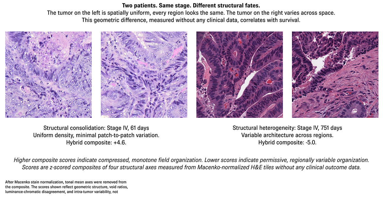
This null result is informative. The average structural deviation of a tumor does not independently predict survival. A tumor where every patch looks equally unusual is not the same as a tumor where some patches are highly consolidated and others are highly disrupted. The distinction between these states, and which is prognostically meaningful, is captured not by the mean but by the distribution of structural states across tumor regions.
6.3 Distribution Beats Mean: Eleven Consistent Axes
A full feature screen of all 120 patient-level axes against overall survival and disease-specific survival identified eleven axes with significant associations in the same direction on both endpoints. These axes span void structure, packing density, gap field behavior, texture variability, and nuclear size irregularity, independent structural dimensions across independent computational layers.
| Axis | OS HR | OS p | DSS HR | DSS p | Biological reading |
|---|---|---|---|---|---|
| mean_gap_rv | 0.620 | 0.0011 | 0.561 | 0.0006 | Protective: void / soft-boundary openness |
| mean_b_rv | 0.625 | 0.0016 | 0.583 | 0.0019 | Protective: baseline void ratio |
| std_tex_contrast_coarse | 0.628 | 0.0070 | 0.551 | 0.0035 | Protective: variability in coarse texture contrast |
| std_etex_homogeneity_coarse | 0.683 | 0.0102 | 0.617 | 0.0042 | Protective: eosin channel texture variability |
| std_blob_size_cv | 0.666 | 0.0107 | 0.645 | 0.0132 | Protective: nuclear size irregularity variability |
| std_etex_contrast_coarse | 0.666 | 0.0196 | 0.590 | 0.0113 | Protective: eosin coarse contrast variability |
| std_htex_energy_coarse | 0.747 | 0.0153 | 0.749 | 0.0266 | Protective: hematoxylin texture energy variability |
| std_htex_entropy_coarse | 0.727 | 0.0361 | 0.685 | 0.0262 | Protective: hematoxylin texture entropy variability |
| mean_b_rho | 1.601 | 0.0014 | 1.711 | 0.0018 | Hazardous: baseline packing density |
| mean_gap_delta_vs_baseline | 1.567 | 0.0031 | 1.628 | 0.0065 | Hazardous: gap field departure from baseline |
| mean_delta_r | 1.408 | 0.0078 | 1.421 | 0.0178 | Hazardous: luminance-chromatic disagreement |
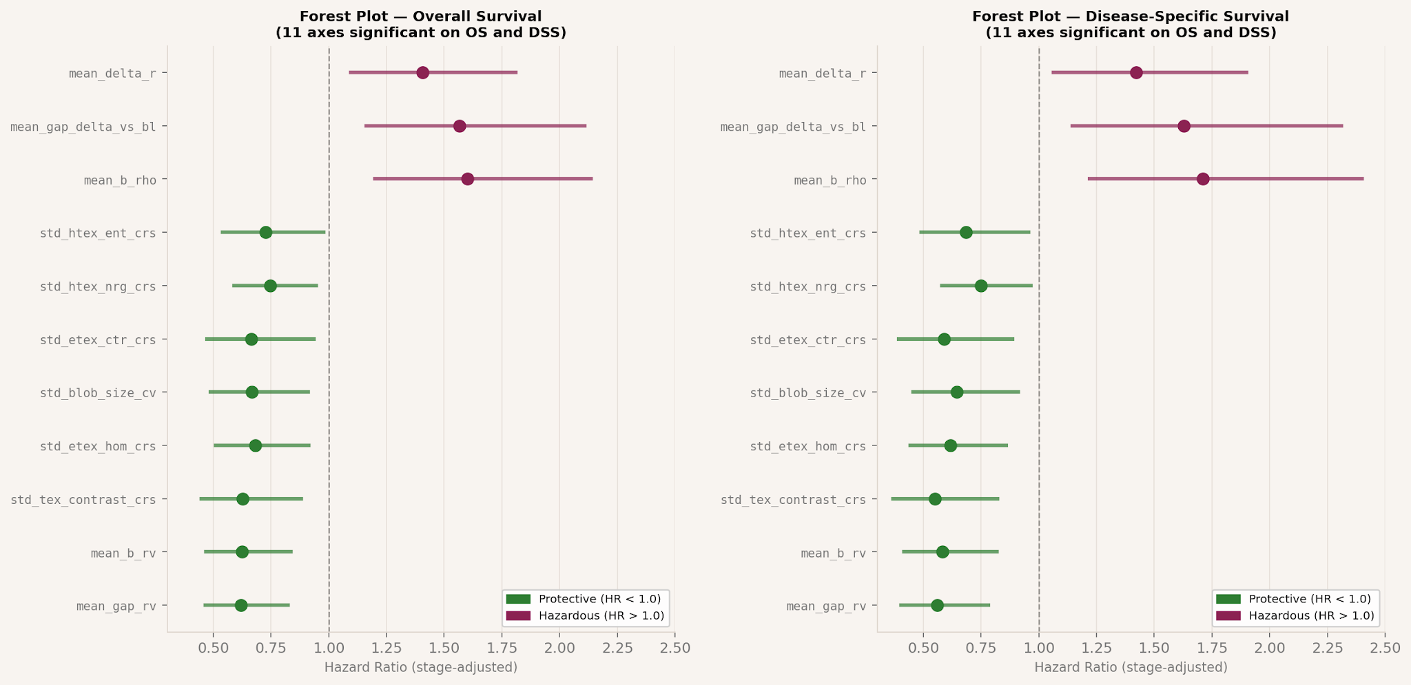
Disease-specific survival shows stronger and more consistent structural associations than overall survival across nearly all axes. This pattern suggests the structural field organization signal is specifically relevant to colorectal cancer mortality rather than confounded by comorbid causes of death.
This finding is consistent with independent work from the deep learning side of computational pathology. (Waqas et al. 2026) demonstrate that standard multiple instance learning frameworks, which aggregate patch-level embeddings by averaging or attention pooling, systematically neglect global tissue architecture and the local spatial context of informative patches, and that augmenting foundation models with explicit spatial encoding improves survival prediction across seven cancer types. Their conclusion, reached through learned representations on whole-slide images, converges with the present finding reached through deterministic geometric measurement on patch samples: the spatial organization of structural states across the tumor carries prognostic information that mean-feature aggregation discards. That two methodologically distinct approaches identify the same gap in the same direction suggests the signal reflects a genuine property of tumor spatial biology rather than an artifact of either measurement strategy.
6.4 Two Structural Field Regimes
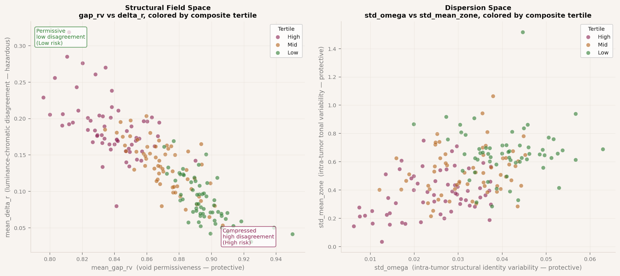
The eleven consistent axes partition into two coherent field states. This structure was not imposed; it emerged from the pattern of associations across the full normalized feature screen.
The permissive field state is characterized by higher void ratios (mean_gap_rv, mean_b_rv), lower packing density, greater regional variability in coarse texture contrast and eosin channel regularity, and more heterogeneous nuclear size distribution across patches. This state is protective across all three survival endpoints.
The compressed field state is characterized by higher baseline packing density (mean_b_rho), greater gap field departure from the luminance baseline (mean_gap_delta_vs_baseline), and elevated luminance-chromatic disagreement (mean_delta_r). When luminance edges exist where color channels do not confirm them, the operational definition of mean_delta_r, the tissue field is structurally dissonant across perceptual channels. This axis was statistically invisible in raw unnormalized data (HR=1.004, p=0.975) and emerges as a significant signal only after normalization removes inter-site staining variation.
The structural story is not that lighter or darker tumors do worse. It is that tumors which have settled into a rigid, compressed, spatially monotone field do worse than tumors that retain regional openness and variation.
6.5 Hybrid Composite Performance
A hybrid composite combining one hazardous mean-geometry axis and three protective axes was evaluated against four pre-specified performance gates. The composite formula is:
Higher scores indicate compressed, less permissive, less regionally variable structural organization. Lower scores indicate open, variable, permissive structural organization.
| Endpoint | HR | 95% CI | p | C-index gain |
|---|---|---|---|---|
| Overall survival (47 events) | 1.687 | [1.261–2.257] | 0.0004 | +0.033 over stage alone |
| Disease-specific survival (36 events) | 1.872 | [1.343–2.608] | 0.0002 | +0.044 over stage alone |
| Progression-free interval (58 events) | 1.385 | [1.069–1.794] | 0.0138 | +0.025 over stage alone |
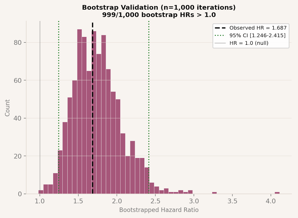
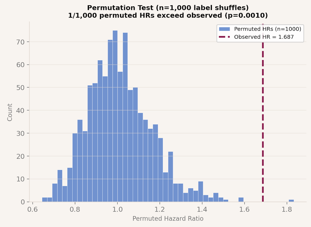
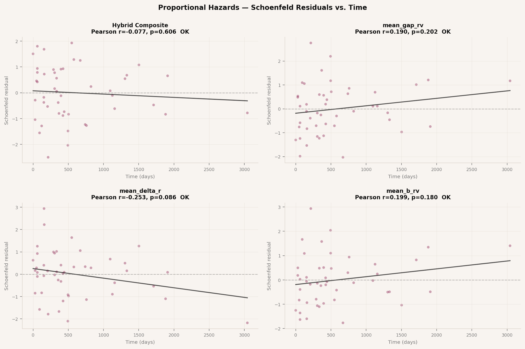
The composite was validated by bootstrap (1,000 iterations; 999/1,000 produced HR > 1.0; bootstrap 95% CI [1.246–2.415]), permutation test (1/1,000 permuted datasets exceeded observed HR; permutation p=0.0010), and jackknife (20 leave-one-out iterations; HR range 1.660–1.754; all 20 iterations HR > 1.0). No single patient drives the composite association. The signal survives mucinous histological subtype adjustment (HR=1.661 vs 1.687 unadjusted, p=0.0006) and passes proportional hazards assumption checking for all contributing axes.
6.6 Tertile Mortality Gradient and Stage Specificity
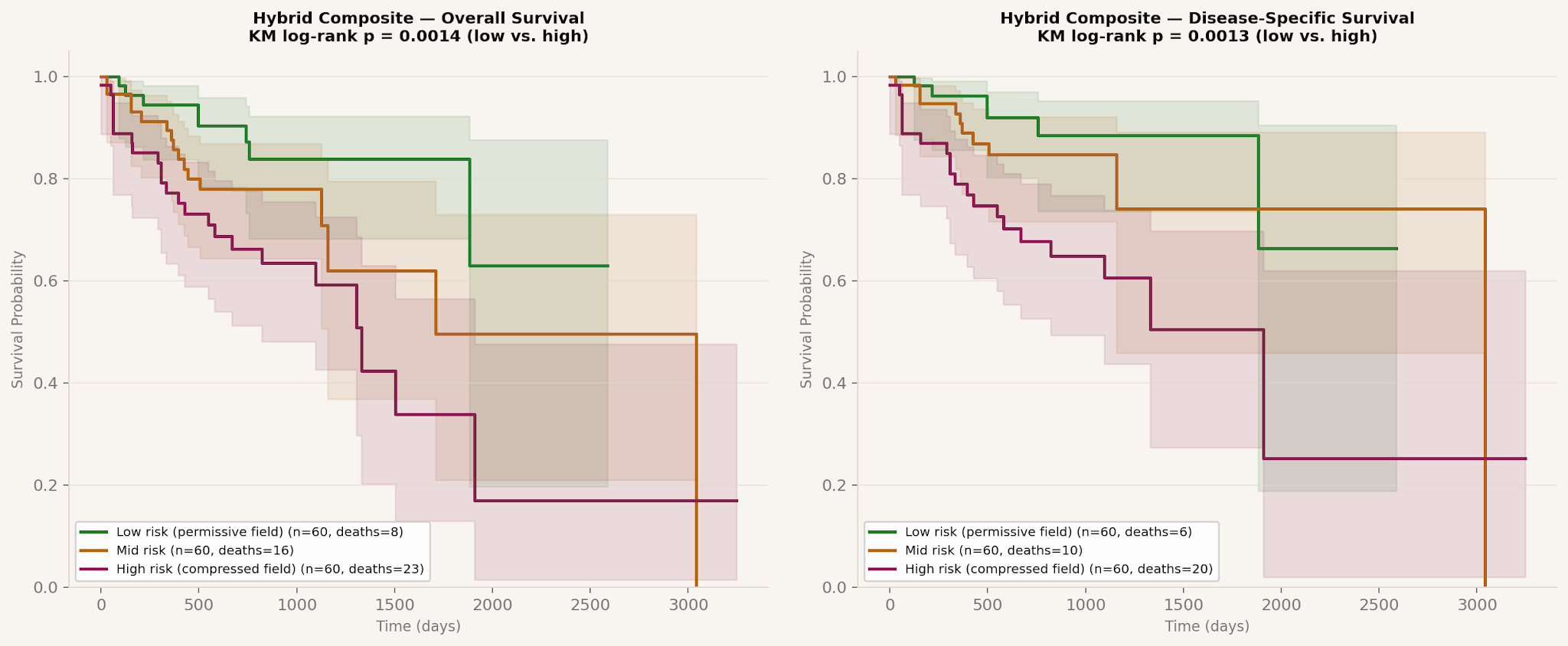
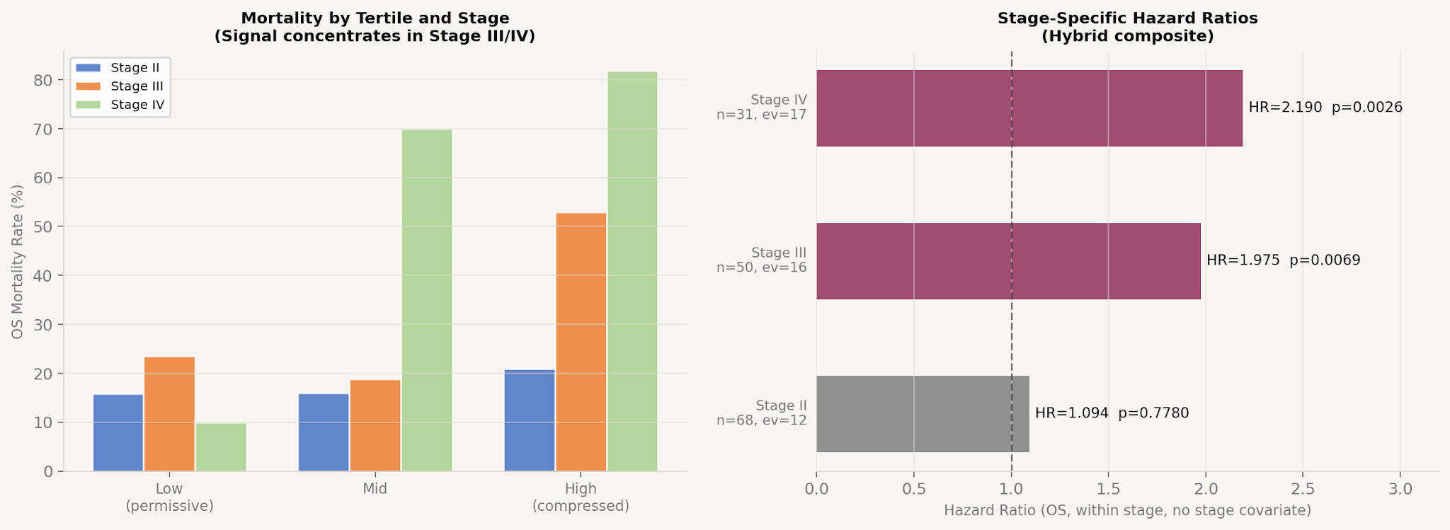
Patients divided into tertiles by composite score show a monotonic mortality gradient across all three endpoints. Observed overall survival mortality spans 13.3% in the low-risk tertile to 38.3% in the high-risk tertile, a 2.9-fold difference in death rate from deterministic structural measurement without any outcome training (KM log-rank p=0.0014).
The composite signal is not equally distributed across the pathological stage. Stage II disease shows no significant composite signal (HR=1.094, p=0.778). The signal concentrates in Stage III (HR=1.975, p=0.007) and Stage IV (HR=2.190, p=0.003) disease, where within-stage outcome heterogeneity is clinically most relevant. This stage specificity argues against the composite functioning as a stage proxy.
7. Discussion
7.1 What the Instrument Uniquely Contributes
Three capabilities distinguish Parallax Pathology from trained computational pathology systems, and none of them are consequences of higher accuracy.
Structural explanation without post-hoc attribution. When this system reports that a patch deviates 4.7 units from its nearest class expectation, primarily because delta_r is elevated, it is reporting that luminance edges exist where color channels do not confirm them. That explanation is not derived from a prediction; it is the measurement itself. Every output is traceable to a specific geometric relationship between specific structural channels. This differs categorically from gradient attribution methods that attach saliency maps to trained predictions after the fact.
Label-agnostic structural positioning. The tissue type is not an input. The system computes Omega against all reference classes simultaneously and returns the nearest class, the own-class distance, and the full per-class distance profile. An unknown tissue type registers as structurally distant from all known classes. The output, which does not fit any known structural regime, is the correct signal for an out-of-distribution observation, not a misclassification.
Deterministic reproducibility. The same image produces identical output on every run, on any hardware, without model weights. This property enables structural comparison across time points, institutions, and preparation methods in ways that embedding-based systems cannot straightforwardly support. No random seed, no stochastic inference, no version drift.
7.2 Implications for Survival Modeling in Computational Pathology
The most important methodological result from the TCGA-COAD analysis is not any specific hazard ratio. It is the consistent pattern: mean structural axes fail to predict survival; distributional and field-organization axes succeed. This pattern repeated across every analytical approach: mean tonal axes collapsed after stain normalization, dispersion axes survived, and the field-organization axes emerged as the strongest normalized signals.
The dominant aggregation strategy in computational pathology collapses tumors into a single representative embedding, typically by averaging patch-level features or pooling patch-level embeddings across a slide. This analysis suggests that step may discard the primary carrier of prognostic information. The signal lives not in what the average patch looks like but in how structural states are distributed across the spatial extent of the tumor.
If validated externally, these findings argue for retaining the variance structure across patches rather than averaging it away, and for modeling the spatial field organization of tumors rather than their average appearance. The computational cost of preserving distributional structure is modest; the potential prognostic benefit appears real.
The two TUM failure modes identified in the tissue classification study (Section 3.4) and the two field regimes identified in the survival analysis (Section 5.4) are expressions of the same underlying observation at different scales. Density loss and directional acquisition in individual deviant patches correspond to the permissive and compressed field states observed at the patient level. A tumor dominated by density-loss failure patches will have high spatial void permissiveness, the permissive field state. A tumor dominated by directional-acquisition failure patches will show compressed, monotone organization, the compressed field state. The geometric through-line from single patch to patient-level survival is coherent.
7.3 The Hybrid Architecture
The appropriate deployment context for Parallax Pathology is alongside trained systems. Foundation models solve the classification problem efficiently and at high accuracy. The question is not whether to replace them, it is what a deterministic measurement layer provides that classification confidence scores do not.
The 58-axis structural feature vector can be concatenated with any foundation model embedding to produce a representation that combines high-accuracy learned features with geometrically interpretable structural measurements. The addition costs computation, running the deterministic pipeline adds time, but produces a richer feature set in which every dimension is interpretable.
Omega used as an out-of-distribution signal alongside a deep classifier produces a system that is both accurate and capable of flagging patches that fall outside the training distribution. In multi-site deployment, where distribution shift between training and clinical populations is common, this asymmetry, the deep classifier is confident on out-of-distribution inputs; the structural measurement is not, is a real capability difference.
The Library of Normals extension points toward the most direct clinical utility: building structural expectation references for normal tissue across organ types, then using Omega deviation as a continuous measure of structural disorganization. The deviation is not a diagnosis. It is a measurement that a clinician, a foundation model, or a downstream statistical model can use as one input among many. To make this concrete: three near-term deployment contexts are well-suited to what the system actually produces. First, quality control and anomaly flagging in pathology pipelines, high-Omega patches are structurally unusual relative to their tissue type, a property useful for slide-level QC, staining artifact detection, and pre-screening before model inference. Second, out-of-distribution detection alongside deployed deep classifiers, a foundation model will assign any input to its nearest training class regardless of how far outside the training distribution that input sits; Omega provides a continuous signal of structural distance from known normal classes that a deep classifier cannot produce. Third, interpretable feature augmentation, the 58 deterministic axes concatenated with learned embeddings give a downstream survival or grading model access to geometrically named dimensions alongside the high-dimensional latent features, enabling feature attribution that points to something a pathologist can look at rather than a pixel region with elevated gradient. None of these require replacing an existing system. They require adding a measurement layer that currently does not exist in standard pathology pipelines.
8. Limitations
The following limitations are documented for direct evaluation by any reader or reviewer.
- FDR correction at 47 events across 120 features is a threshold this study was never sized to meet, it would require approximately 400–500 events to have adequate power for FDR-corrected single-feature confirmation at this feature count. The absence of FDR-significant individual features is therefore expected and uninformative about whether signal exists. The relevant evidence is elsewhere: eleven axes align in the same direction across two independent endpoints (OS and DSS), the composite HR of 1.687 is stable under bootstrap (999/1,000 iterations HR > 1.0) and permutation (1/1,000 shuffled datasets exceeded observed), and the strongest emerging signal, mean_delta_r, has a mechanistic explanation for why it appears specifically after stain normalization rather than in raw data. Taken together, this is an exploratory signal with enough coherence and stability to justify external validation. It is not confirmed science. External replication in an adequately powered independent cohort is the only test that matters next.
- Same-cohort composite evaluation. The hybrid composite was selected and evaluated on the same 180-patient cohort. Optimistic bias is present and its magnitude is unknown. The bootstrap and permutation tests confirm the signal is not a sampling artifact; they do not eliminate selection bias. External replication will likely produce smaller effect sizes.
- Random tile sampling. Approximately 50 random tiles per patient is a sample, not a spatial map. Structural variability metrics reflect patch-to-patch variation in a random sample rather than systematic spatial heterogeneity. True spatial field organization measurement requires spatially stratified tiling from source whole-slide images.
- Tile composition is not labeled. Tiles processed as tumor-containing may include substantial stromal or immune tissue. Standard deviation axes measuring within-patient variability may partly reflect variation in tissue compartment sampling rather than tumor-intrinsic structural heterogeneity. This cannot be resolved without tile-level compartment classification.
- Scale ceiling at the benchmark level. The system measures structural properties at the cellular and tissue-zone level. Features requiring larger fields of view, gland spacing regularity, tumor budding at the invasive front, spatial extent of desmoplastic reaction, are not captured at 224px and 0.5 microns per pixel. Architectural grading questions require multi-scale analysis or larger input fields.
- EBHI-SEG class imbalance. Normal (n=76) and Serrated (n=58) have substantially fewer patches than other EBHI classes (n=186–200). The 5.6 percentage point difference between full-dataset and balanced accuracy is documented. The floor under fully balanced conditions is approximately 62%; the Spearman correlations and Kruskal-Wallis statistics are not materially affected by class imbalance.
- No external normalization on EBHI-SEG. Cross-dataset absolute Omega comparison between CRC-VAL and EBHI is not valid without matching preparation methods. Within-dataset deviation scores are valid; cross-dataset comparisons require preparation-matched references.
- Reference constructed from evaluation cohort. The Omega structural expectation reference for TCGA-COAD was built from the same 180-patient cohort used for survival analysis. This creates reference leakage that biases toward internal structural consistency. A reference built from an independent normal tissue dataset would provide a cleaner evaluation.
- Preparation sensitivity of texture axes. GLCM texture axes at fine scale (sigma=2) are sensitive to scanner point spread function, compression artifacts, and staining intensity variation in ways that orientation coherence and void ratio are not. Cross-site application of the full 58-axis reference requires preparation-matched reference construction.
- Authorship on visual validation. The biological interpretations offered for high and low Omega patches are made by a researcher with familiarity with histopathology concepts, not by a board-certified pathologist. The geometric findings are real and reproducible; the biological readings should be treated as hypotheses pending expert pathologist review.
9. Future Work
- External survival validation. The hybrid composite and the eleven consistent axes must be evaluated in an independent colorectal cancer cohort with Macenko normalization applied before any prognostic claim can be made. TCGA-READ (rectal cancer) provides the most accessible independent target.
- Spatially stratified tiling. Replacing random tile sampling with a grid-based or region-of-interest sampling strategy would provide a true spatial map of structural field organization across the tumor. This is the most direct methodological improvement for survival modeling.
- Tile composition labeling. Classifying tiles by compartment (tumor, stroma, immune-predominant) before computing structural features would allow clean separation of tumor-intrinsic architecture from microenvironmental signals.
- EBHI-SEG external validation and outcome correlation. The dysplasia progression signal requires correlation with clinical outcomes, like recurrence, progression to cancer, and treatment response, to establish translational relevance. A prospective validation using continuous molecular markers (Ki-67 index, MSI status) as ground truth rather than categorical grade labels would establish whether structural disorganization scores track biological state independently of pathologist-assigned grade.
- Library of Normals. Building structural expectation references for breast, lung, kidney, and skin using normal tissue only. Each reference would encode the structural laws of that tissue type. Pathological cases surface as deviations from the normal reference without requiring labeled pathological examples.
- Molecular subtype correlation. Correlating the two structural field regimes with MSI status, KRAS/BRAF mutation status, and consensus molecular subtypes would establish whether geometric field organization tracks known biological states.
- Foundation model integration. Concatenating the 58-axis structural vector with UNI or CONCH embeddings as a combined feature representation for survival modeling. The hybrid carries both high-accuracy learned features and geometrically interpretable structural measurements.
- Multi-scale analysis. Applying the measurement framework at multiple patch sizes (224px, 512px, 1024px) to capture structural properties at nuclear, cell-arrangement, and gland-architecture scales simultaneously.
- Longitudinal structural drift. Applying Omega to serial biopsies with known outcomes to test whether tissue drifting toward a pathological state shows increasing structural deviation before a defined histological diagnosis is possible.
References
- Chen, R.J., et al. (2024). Towards a general-purpose foundation model for computational pathology. Nature Medicine.
- Lu, M.Y., et al. (2024). A visual-language foundation model for computational pathology (CONCH). Nature Medicine.
- Holzinger, A., et al. (2019). Causability and explainability of AI in medicine. WIREs Data Mining and Knowledge Discovery.
- Srinidhi, C.L., et al. (2021). Deep neural network models for computational histopathology: A survey. Medical Image Analysis.
- Parrish, R. (2025). Visual Thinking Lens: A geometric kernel for compositional analysis of visual art. artistinfluencer.com.
- Kotani, A., et al. MATISSE: Retinal Simulation Framework. github.com/atsu-kotani/Matisse. DOI: 10.5281/zenodo.14205776.
- Ruifrok, A.C., Johnston, D.A. (2001). Quantification of histochemical staining by color deconvolution. Analytical and Quantitative Cytology and Histology.
- Kather, J.N., Halama, N., Marx, A. (2018). 100,000 histological images of human colorectal cancer and healthy tissue. Zenodo. https://doi.org/10.5281/zenodo.1214456
- Macenko, M., et al. (2009). A method for normalizing histology slides for quantitative analysis. ISBI.
- Kather, J.N., et al. (2020). Predicting survival from colorectal cancer histology slides using deep learning. PLOS Medicine. Zenodo DOI: 10.5281/zenodo.3784345.
- Liu, J., et al. (2018). An integrated TCGA pan-cancer clinical data resource. Cell, 173(2):400-416.
- Swanton, C. (2012). Intratumor heterogeneity: evolution through space and time. Cancer Research, 72(19):4875-4882.
- Selvaraju, R.R., et al. (2017). Grad-CAM: Visual explanations from deep networks. ICCV.
- Li, C., Shi, L., Hu, W. et al. (2022). Enteroscope Biopsy Histopathological H&E Image Dataset for Image Segmentation Tasks (EBHI-Seg). Zenodo. First release: 11-11-2022.
- Waqas, M., Bandyopadhyay, R., Showkatian, E., Muneer, A., Zafar, A., Alvarez, F.R., et al. (2026). The next layer: augmenting foundation models with structure-preserving and attention-guided learning for local patches to global context awareness in computational pathology. npj Precision Oncology, 10, 109. https://doi.org/10.1038/s41698-026-01312-5
Data Sets:
- Kather, J. N., Krisam, J., Charoentong, P., Luedde, T., Herpel, E., Weis, C. A., Gaiser, T., Marx, A., Valous, N. A., Ferber, D., Jansen, L.,
- Reyes-Aldasoro, C. C., Zörnig, I., Jäger, D., Brenner, H., Hoffmeister, M., & Halama, N. (2019). Predicting survival from colorectal cancer histology slides using deep learning: A retrospective multicenter study. PLOS Medicine, 16(1), e1002730. doi.org
- GTEx Consortium. (2020). The GTEx Consortium atlas of genetic regulatory effects across human tissues. Science, 369(6509), 1318–1330. doi.org
- Shi, L., Li, X., Hu, W., Chen, H., Chen, J., Fan, Z., … & Li, C. (2023). EBHI-Seg: A novel enteroscope biopsy histopathological hematoxylin and eosin image dataset for image segmentation tasks. Frontiers in Medicine, 10, 1114673. doi.org
Appendix A: Mathematical Specification
A.1 Kernel Primitive Formulas
| Primitive | Formula | Geometric meaning |
|---|---|---|
| Δx, Δy | Σ(pᵢ·xᵢ)/Σpᵢ normalized to [−0.5, 0.5] | Gradient-weighted centroid in x and y |
| rᵥ | Σ1[pᵢ < τ]/N (τ = 0.18) | Void ratio; fraction of field below void threshold |
| μ | Σ1[pᵢ ≥ Q₇₅]·pᵢ/Σpᵢ | Cohesion; fraction of energy in top-quartile pixels |
| SDI | mean(√((xᵢ−cx)²+(yᵢ−cy)²))/diag for active pᵢ | Spatial dispersion; mean distance from centroid |
| ρᵣ | N_active / A_convex_hull | Packing density; active pixels to convex hull area |
| X | Σ1[peripheral]·pᵢ/Σpᵢ (outer 15% band) | Peripheral pull; mass fraction in outer border band |
| θ | 1 − H(angles)/log₂(8) | Orientation coherence; 0=isotropic, 1=aligned |
| dₛ | mean chamfer distance inside active region | Structural thickness; approximates ridge/duct width |
A.2 Coherence Score Formulas
Omega (mask agreement): Omega = (1/|P|) · Σ_{(i,j)∈P} √((dxᵢ−dxⱼ)²+(dyᵢ−dyⱼ)²), where P is all pairs of non-degenerate non-combined masks and dxᵢ, dyᵢ are centroid coordinates.
Gamma (boundary permissiveness): Γ = rᵥ_confirmed − rᵥ_cone_max. High Gamma means more structure lives beyond the conservative luminance boundary.
Delta-r (luminance-chromatic disagreement): Δᵣ = rᵥ_confirmed − rᵥ_baseline. High delta_r = luminance edge structure not confirmed by color opponency.
Beta (blind spot mass): B = 1 − rᵥ_blind_spot. High Beta = color structure where luminance sees nothing.
A.3 Configuration Parameters
Appendix B: Claims Boundary
What This Paper Claims
- The system produces deterministic, reproducible geometric measurements from H&E image patches with no trained parameters
- The 58-axis system achieves 91.5% nine-class linear accuracy on CRC-VAL-HE-7K using LDA with 5-fold stratified CV, reproducible from published batch results
- The emergence gap of 16.3 percentage points between the best standalone layer and the full system confirms that the layers encode genuinely complementary structural information
- Structural centers emerge within individual unlabeled datasets across independent donors and preparation methods
- Eleven structural axes show directionally consistent significant associations with both OS and DSS in TCGA-COAD after Macenko normalization and stage adjustment
- The hybrid composite stratifies 180 TCGA-COAD patients with OS HR=1.687 (p=0.0004), confirmed by bootstrap, permutation, and jackknife validation
- Signal concentrates in Stage III and IV disease and is not explained by mucinous histological subtype
What This Paper Does Not Claim
- That any survival finding survives FDR correction or constitutes a validated biomarker
- That the composite HR will replicate at the same magnitude in an external cohort
- That high Omega correlates with pathological grade, malignancy, or any clinical outcome, this has not been tested as a direct correlation
- That the system replaces or competes with foundation models on classification accuracy
- That the system is clinically validated or ready for any clinical application
- That the biological interpretations of structural failure modes have been validated by expert pathologist review
- That the 91.5% accuracy generalizes beyond CRC-VAL-HE-7K to other datasets, scanners, or staining protocols without reference recalibration
All data, source code, and result files are available on request. ORCID: 0009-0008-9781-7995.
Appendix C: Statistical Validation and Robustness
This appendix documents the full suite of stability checks, sensitivity analyses, and robustness tests applied to the survival analysis findings in Section 5. It is organized in the order a reviewer would want to work through it: composite stability first, then individual axis robustness, then normalization impact, then the full feature screen.
C.1 Bootstrap Validation of the Hybrid Composite
One thousand bootstrap samples were drawn with replacement from the 180-patient cohort. For each sample, the composite was re-z-scored and a stage-adjusted Cox proportional hazards model was fit. The distribution of resulting hazard ratios is summarized below.
| Validation metric | Result |
|---|---|
| Observed OS HR (stage-adjusted) | 1.687 [1.261–2.257], p=0.0004 |
| Bootstrap median HR (n=1,000) | 1.725 |
| Bootstrap 95% CI | [1.246–2.415] |
| Bootstrap iterations with HR > 1.0 | 999/1,000 (99.9%) |
| Upward bias in point estimate | None detected (bootstrap median 1.725 vs observed 1.687) |
The bootstrap 95% confidence interval lies entirely above 1.0. The bootstrap median HR of 1.725 is consistent with the observed HR of 1.687, indicating no substantial upward bias in the point estimate. The signal is not a function of any particular sample draw from the 180-patient cohort.
C.2 Permutation Test
One thousand permutation tests were performed by randomly shuffling both OS event status and OS time simultaneously across patients, then fitting the same stage-adjusted Cox model on the shuffled data. This tests whether the observed association could arise by chance from the correlation structure of the feature space alone.
| Permutation metric | Result |
|---|---|
| Permutation tests run | 1,000 (simultaneous shuffle of event status and time) |
| Permuted HRs exceeding observed | 1/1,000 |
| Permutation p-value | 0.0010 |
| Interpretation | Observed association is not a chance finding in this dataset |
The permutation test confirms that the composite association is not explainable by random correlation between the 58-axis feature structure and the outcome data. Only 1 of 1,000 permuted datasets produced a hazard ratio meeting or exceeding the observed value.
C.3 Jackknife (Leave-One-Out) Validation
Twenty leave-one-out iterations were performed by removing one patient at a time from a randomly selected sample of 20 patients and refitting the Cox model on the remaining 179 patients. This tests whether any single patient is driving the composite association.
| Jackknife metric | Result |
|---|---|
| Iterations run | 20 leave-one-out removals |
| HR range across iterations | 1.660–1.754 |
| Mean HR across iterations | 1.691 |
| Standard deviation | 0.023 |
| Iterations with HR > 1.0 | 20/20 (100%) |
C.4 Mucinous Histological Subtype Adjustment
Mucinous adenocarcinoma (n=16, 8.9% of cohort) is a histologically distinct subtype with different structural organization than conventional adenocarcinoma. The composite and primary contributing axes were refit with mucinous status as an additional binary covariate alongside stage to test for confounding.
| Feature | HR (stage only) | HR (stage + mucinous) | p | Assessment |
|---|---|---|---|---|
| Hybrid composite | 1.687 | 1.661 | 0.0006 | Signal unchanged |
| mean_gap_rv | 0.620 | 0.622 | 0.0012 | Signal unchanged |
| mean_delta_r | 1.408 | 1.397 | 0.0098 | Signal unchanged |
C.5 Proportional Hazards Assumption
The Cox proportional hazards model assumes that hazard ratios are constant over time. This assumption was checked for the hybrid composite and three primary contributing axes using Schoenfeld residuals. Pearson and Spearman correlations between residuals and survival time were tested; significant correlation indicates time-varying hazard ratio behavior.
| Feature | Pearson p | Spearman p | Assessment |
|---|---|---|---|
| Hybrid composite | 0.606 | 0.502 | No violation |
| mean_gap_rv | 0.202 | 0.106 | No violation |
| mean_delta_r | 0.086 | 0.282 | No violation (Pearson marginal; Spearman clear) |
| mean_b_rv | 0.180 | 0.188 | No violation |
C.6 Normalization Impact: Before and After
Macenko stain normalization was applied to all tiles prior to feature computation. This was not cosmetic. The normalization sensitivity analysis on a four-patient subset (two low structural deviation patients, two high) established which axes survive normalization as architectural signals and which collapse as preparation chemistry artifacts. Those verdicts guided the composite construction and determined which findings from this paper can be stated as architectural rather than staining-driven.
| Axis | Raw OS HR | Raw OS p | Normalized OS p | Verdict |
|---|---|---|---|---|
| mean_highlight_mass | 1.429 | 0.005 | 0.300 | WITHDRAWN — preparation-sensitive |
| mean_mean_zone | 1.349 | 0.011 | 0.316 | WITHDRAWN — preparation-sensitive |
| std_omega | — | 0.019 | 0.108 (trend) | DIRECTION PRESERVED — used in composite |
| std_mean_zone | — | 0.021 | 0.167 (trend) | DIRECTION PRESERVED — used in composite |
| mean_gap_rv | — | 0.294 | 0.001 | EMERGED after normalization |
| mean_delta_r | 1.004 | 0.975 | 0.008 | EMERGED after normalization — was invisible in raw data |
The emergence of mean_delta_r as a significant signal specifically after normalization is the single most striking individual finding in the survival analysis. Luminance-chromatic disagreement was buried under inter-site staining variation in raw multi-site TCGA data. Normalization removed the chemistry layer and the architectural signal became detectable. The axis measures structural incoherence between luminance and color channel organization, a property of tissue architecture independent of staining preparation.
C.7 Composite Candidate Selection: Full Gate Results
Three composite candidates were pre-specified after the normalization sensitivity analysis: a dispersion-only composite (C_disp), an extended mean-geometry composite (C_mean+), and the hybrid composite (C_hybrid). All were evaluated against a pre-defined gate framework applied uniformly before any survival model was fit on the full cohort.
Gate definitions: Gate 2, Stage-adjusted OS HR > 1.30 AND p < 0.01. Gate 3, C-index gain over stage-alone model of at least 0.02. Gate 4, KM log-rank p < 0.01 (low vs. high tertile) with monotonic mortality gradient.
| Composite | OS HR | OS p | DSS HR | DSS p | C-gain OS | KM p | Gates G2/G3/G4 |
|---|---|---|---|---|---|---|---|
| C_disp (Dispersion) | 1.426 | 0.028 | 1.599 | 0.009 | +0.018 | 0.033 | Fail / ~ / ~ |
| C_mean+ (Mean-geom+) | 1.586 | 0.001 | 1.711 | 0.001 | +0.037 | 0.009 | Pass / Pass / Pass |
| C_hybrid (SELECTED) | 1.687 | 0.0004 | 1.872 | 0.0002 | +0.033 | 0.0014 | Pass / Pass / Pass |
C.8 Full Feature Screen: All Significant OS Associations
All 120 patient-level structural features (60 mean axes and 60 standard deviation axes) were screened against overall survival using stage-adjusted Cox regression. The table below shows all features with p < 0.05. No feature survives Benjamini-Hochberg FDR correction at q < 0.05 given 47 OS events across 120 tests.
| Axis | OS HR | 95% CI | p | Direction |
|---|---|---|---|---|
| mean_gap_rv | 0.620 | [0.466–0.825] | 0.0011 | Protective |
| mean_b_rho | 1.601 | [1.199–2.137] | 0.0014 | Hazardous |
| mean_b_rv | 0.625 | [0.467–0.837] | 0.0016 | Protective |
| mean_gap_delta_vs_baseline | 1.567 | [1.163–2.110] | 0.0031 | Hazardous |
| std_tex_contrast_coarse | 0.628 | [0.448–0.881] | 0.0070 | Protective |
| mean_delta_r | 1.408 | [1.094–1.811] | 0.0078 | Hazardous |
| std_etex_homogeneity_coarse | 0.683 | [0.510–0.914] | 0.0102 | Protective |
| std_blob_size_cv | 0.666 | [0.488–0.910] | 0.0107 | Protective |
| mean_tex_contrast_coarse | 0.671 | [0.492–0.915] | 0.0118 | Protective |
| std_htex_energy_coarse | 0.747 | [0.590–0.945] | 0.0153 | Protective |
| std_etex_contrast_coarse | 0.666 | [0.473–0.937] | 0.0196 | Protective |
| std_htex_entropy_coarse | 0.727 | [0.539–0.979] | 0.0361 | Protective |
C.9 Multiple Testing Context
120 patient-level features were tested against OS with 47 events. Under Benjamini-Hochberg FDR correction at q < 0.05, no individual feature survives. This is the correct and expected result at this sample size and event count, and it is stated directly in the paper.
The argument against chance explanation does not rest on individual p-values. It rests on three converging lines of evidence:
- Cross-endpoint consistency. Eleven axes are significant on both OS and DSS in the same direction. The probability of this occurring by chance for eleven independent features across two endpoints is substantially lower than any individual p-value suggests.
- Biological coherence. The eleven axes form two interpretable biological groupings, protective openness and variability axes, and hazardous compression and disagreement axes, rather than a random scatter across the feature space.
- Composite stability. Bootstrap, permutation, and jackknife validation confirm the composite signal is not a sampling artifact. The permutation test establishes that the association exceeds what the correlation structure of the feature space alone would produce.
None of these arguments eliminate the need for external validation. They establish that the pattern of associations is more coherent and stable than FDR-uncorrected p-values read in isolation would suggest.
Appendix D: Anticipated Questions and Honest Responses
This appendix addresses the questions a rigorous reviewer, statistician, or clinical collaborator would raise about this work. They are answered directly rather than deflected. Science that does not document its own failure modes has not been done honestly.
D.1 Anticipated Objections: Survival Analysis
Q: You selected composite components from the same data you used to evaluate the composite.
Correct. This is documented explicitly throughout the paper. Two of four C_hybrid components (std_omega, std_mean_zone) were identified as normalization-stable before the full normalized run was executed, they carry partial pre-specification. Two components (mean_delta_r, mean_gap_rv) emerged from the normalized feature screen and are post-hoc. The bootstrap and permutation tests confirm the composite signal is not a sampling artifact, but they do not eliminate optimistic bias. External validation is required before the HR numbers can be cited as performance claims. This is stated in every section that reports composite results.
Q: No feature survives FDR correction. These findings are noise.
FDR correction at 47 events across 120 features is a threshold that would reject almost any real signal at this sample size, as expected. The argument against noise is not p-value magnitude but cross-endpoint consistency, biological coherence, and composite stability under resampling. Eleven axes aligning in the same direction across two independent endpoints (OS and DSS) is a pattern that chance alone produces infrequently. That said, this objection is not dismissed and it is the primary reason external validation is the stated highest-priority next step. These findings are explicitly labeled exploratory throughout.
Q: TCGA-COAD is a multi-site dataset with massive staining variation. Your results reflect staining artifacts.
This was the primary concern motivating Macenko normalization. The normalization sensitivity analysis confirmed that tonal mean axes (highlight_mass, mean_zone) are preparation-sensitive and collapsed after normalization; those results are not claimed. The surviving and emerging signals are geometric and texture axes with lower sensitivity to staining chemistry. The emergence of mean_delta_r specifically after normalization (p=0.975 raw, p=0.008 normalized) is the clearest counter-evidence to the artifact interpretation: if the signal were a staining artifact, it would be stronger in raw data, not invisible in it. The mucinous subtype adjustment and cross-endpoint consistency further reduce the artifact explanation.
Q: Fifty random tiles per patient does not measure spatial tumor structure.
Correct, and this is stated directly in the limitations. Fifty random tiles per patient is a sample, not a spatial map. The standard deviation axes measuring within-patient variability reflect patch-to-patch variation in a random sample, not systematic spatial heterogeneity. This is a structural limitation of the current approach and does not invalidate the findings, it means the findings likely underestimate the true spatial field organization signal rather than overestimate it. Spatially stratified tiling is listed as the highest-priority methodological improvement.
Q: Tile composition is not labeled. Your structural variability measures may reflect stromal or immune sampling, not tumor architecture.
Correct. A tile labeled as tumor-containing may include substantial stromal or immune tissue. Within-patient variability metrics may partly reflect variation in tissue compartment sampling rather than tumor-intrinsic structural heterogeneity. This cannot be resolved without tile-level compartment classification. It is a known limitation documented in both the main text and the limitations section. If anything, this limitation would tend to dilute a genuine tumor-architectural signal by adding noise from compartment sampling variation, making the observed associations conservative rather than inflated.
Q: Stage IV patients have more events and more structurally variable tissue. The composite is a stage proxy.
Stage is included as a covariate in all Cox models reported. The composite adds incremental discrimination beyond stage (C-index gain +0.033 OS, +0.044 DSS). The within-stage analysis uses no stage covariate and still shows strong Stage III and IV effects (HR=1.975 and 2.190 respectively). The Stage II null result (HR=1.094, p=0.778) is the most important counter-evidence: a stage proxy would show signal in Stage II, where outcome variation exists and stage is by definition heterogeneous. The absence of signal in Stage II argues specifically against a stage-proxy explanation.
Q: The Omega reference was built from the same cohort used for analysis.
Correct. This creates reference leakage that biases toward internal structural consistency and may compress the variance of Omega-derived features. Raw structural axes (gap_rv, delta_r, b_rv, b_rho) do not depend on the Omega reference and are not affected by this. The Omega-derived features (mean_omega, std_omega) are the most affected. std_omega is used in the composite but only carries trend-level significance on its own after normalization, the composite HR is not primarily driven by the Omega-dependent components. An independent reference would provide a cleaner evaluation and is documented as future work.
D.2 Anticipated Objections: Tissue Classification
Q: 91.5% accuracy is substantially below foundation model performance (95–99%). Why report this as a validation?
The 91.5% figure is offered as evidence that the deterministic metric space has real geometric structure, that tissue types occupy linearly separable regions in the measurement space, not as a competitive classification performance claim. A system with no learned parameters reaching 91.5% on a nine-class benchmark establishes that the structural measurement is capturing something real. The gap to foundation models (5–8 percentage points) reflects genuinely non-geometric information that the interpretability requirement excludes. These are not the same question answered differently; they are different questions. The paper states this directly in Section 2.3.
Q: The feature set was selected by greedy search on the evaluation dataset. This inflates accuracy.
The greedy selection used five-fold stratified cross-validation on the same dataset, which protects against patch-level overfitting within the dataset. It does not protect against distributional selection bias toward this specific benchmark. Performance on a different colorectal dataset with a different scanner, staining protocol, or patient population should be expected to be lower until validated. This is acknowledged in Appendix B and in the main text.
Q: STR at 74.5% is still the weakest clinical class. This indicates the system has not solved the stroma classification problem.
Accurate. STR is the weakest clinical class and the dominant remaining confusion (61 combined MUS-STR errors) is a structural adjacency at 224px that is not fully correctable with additional features. Visual inspection of deviant MUS and STR patches confirms that a subset is genuinely ambiguous at 112-micron field width; the organizational context that would resolve the classification is outside the frame. This is a scale limitation, not a feature limitation. The ablation confirms that every layer contributes to STR performance; the system has extracted most of what a single 224px patch can provide. The problem at this scale is not solvable by adding more axes.
D.3 Anticipated Objections: Instrument and Generalization
Q: The biological interpretations of failure modes were not made by a pathologist. They may be wrong.
Correct. The biological interpretations, mucinous differentiation, desmoplastic reaction, and lymphocytic margin invasion, are offered by a researcher with familiarity with histopathology concepts, not a board-certified pathologist. The geometric findings are real and reproducible regardless of their biological interpretation. The interpretations are the most plausible readings of the geometric signatures, not pathological diagnoses. Expert pathologist review of the high and low Omega image grids is explicitly offered as an open invitation, and independent pathologist co-authorship is identified as the appropriate validation step for biological interpretation claims.
Q: The frame-memory distinction is not novel. Many anomaly detection frameworks separate measurement from reference.
The abstract principle of separating a fixed measurement coordinate system from an exchangeable reference is not claimed as novel. The contribution is the specific instantiation: a deterministic, interpretable, six-dimensional geometric coordinate system with biologically meaningful axes, validated on histology tissue, with axis-level deviation decomposition that produces explanations in terms clinicians recognize. The novelty is in the instrument and its validated behavior, not in the abstract separation principle.
Q: This is feature engineering plus a distance metric plus LDA. The technical novelty is incremental.
Fair. At the component level: the kernel primitives are classical geometric measures, the distance metric is variance-weighted Euclidean, and the classifier is LDA. None of these are novel in isolation. The paper does not claim they are. The contribution is not in the components but in three things the combination demonstrates. First, that a deliberately constrained, interpretable coordinate system, one where every axis has a named biological reading, can reach 91.5% accuracy on a nine-class histology benchmark without any training data, which establishes that tissue types have genuine geometric structure that does not require learned representations to detect. Second, that the same coordinate system generalizes across tissue types, fixation methods, and donors without retraining, which a learned system cannot do without retraining. Third, that the deviation scalar from this system carries a survival-associated signal in colorectal cancer that survives stain normalization and is grounded in named geometric axes rather than latent features. Incremental technical novelty in service of a useful capability is not the same as no novelty. The honest framing is: this is a carefully designed classical system that has been made to work well on a problem where classical systems are rarely applied seriously, and that produces a specific capability, interpretable geometric explanation, that current state-of-the-art systems do not provide.
Q: The system is training-free but the 58 axes were hand-designed and tuned. That is just overfitting at the design level rather than the training level.
Partially correct, and worth engaging directly. The 58 axes were designed with histology in mind and iteratively extended based on performance on CRC-VAL-HE-7K. That is a form of human-guided optimization that is not the same as gradient descent but shares its directional logic: the designer made choices that improved measured performance on a specific dataset. Three things distinguish this from standard overfitting. First, the axes are not free parameters adjusted to minimize loss, they are named geometric constructs with fixed computational definitions. Adding a new axis requires justifying what it measures, not just that it improves a number. Second, the ablation study demonstrates that every layer added to the 58-axis set improved performance on held-out cross-validation folds, and that no axis among the remaining unused columns added signal, the selection was exhaustive rather than cherry-picked. Third, and most importantly, the GTEx cross-dataset validation demonstrates that the same axes produce meaningful structural centers and biologically coherent deviation fields in completely independent data under a different preparation method, without any adjustment. A hand-tuned system that truly overfits to one dataset should not generalize cleanly across fixation methods to produce the correct tissue-type ordering on void ratio and orientation coherence. The fair summary: the design choices concentrate signal in ways that reflect the designer's understanding of tissue geometry. That is not the same as overfitting, but it means the claim of zero human prior is false, and the paper does not make that claim.
Q: Three GTEx donors does not constitute a generalization study.
Correct. The GTEx analysis demonstrates that the structural center emergence property holds in three independent cases across a different fixation method. It does not characterize the distribution of structural parameters across the GTEx population, does not provide confidence intervals on normal colon structural norms, and does not constitute a population-level generalization claim. The section is titled cross-dataset generalization, not cross-population validation. Its contribution is demonstrating that the frame-memory separation works in practice across preparation methods, not establishing the boundaries of generalization.
Q: The 68.1% six-class accuracy on EBHI-SEG is substantially below 91.5% on CRC-VAL. Does this indicate the system degrades on harder tasks?
The two numbers are not comparable. CRC-VAL separates geometrically distinct tissue types across a wide structural space. EBHI-SEG grades a continuous biological progression where adjacent classes overlap by design. The correct EBHI metric is 84.3% correct-or-adjacent and Spearman r=0.716, a system producing random grade assignments would show r near zero and correct-or-adjacent near 50%. The 68.1% figure without ordinal context misrepresents what the task requires and what the instrument is doing.
D.4 Findings That Are Withdrawn
Earlier versions of this analysis produced findings that do not survive normalization or have been identified as methodologically compromised. They are documented here so that any earlier-circulated materials are not cited without this context.
| Finding / claim | Why it is withdrawn |
|---|---|
| mean_highlight_mass as standalone survival predictor (OS HR=1.429, p=0.005 in raw data) | Non-significant after normalization (p=0.300). Preparation-sensitive staining proxy. Not claimed. |
| mean_mean_zone as survival predictor (DSS HR=2.635, p<0.0001 in raw data) | Non-significant after normalization (OS p=0.316, DSS p=0.979). Collapsed under normalization. Not claimed. |
| Original TCI composite (mean_highlight_mass − std_omega − std_tex_contrast − std_mean_zone) | The primary component (mean_highlight_mass) was a staining proxy. Original composite withdrawn. Replaced by C_hybrid with normalization-stable components. |
| gamma (boundary permissiveness) as survival axis | Large pre-normalization delta collapsed to non-significance after normalization. Not included in claims. |
| DSS concordance 0.850 reported in earlier draft | Updated to 0.808 from normalized analysis with corrected model configuration. Earlier figure should not be cited. |
D.5 Findings That Are Robust and Unlikely to Change
Some findings are more robust than the accuracy and hazard ratio numbers themselves. These would be expected to replicate directionally under any reasonable re-evaluation.
- Rank order of tissue classification difficulty. STR will be the hardest clinical class under any reasonable feature set applied to colorectal tissue at this scale. MUS will be adjacent. ADI will be easy. This reflects tissue biology. No feature addition at 224px will change this ordering fundamentally.
- The emergence result. Adding texture to geometry improves classification performance on this task. The specific magnitude (16.3pp) may vary across evaluations, but the qualitative direction is robust. Individual layers encode genuinely different structural properties.
- The MUS/STR confusion as a scale problem. The remaining cross-errors between MUS and STR are concentrated at tissue compartment boundaries where organizational context is outside the 224px frame. This is not addressable by additional features at this scale.
- The preparation sensitivity hierarchy. Geometric axes (k_rv, theta) are more stable across preparation methods than luminance and chemical texture axes. This is grounded in the physics of the measurements. It would be expected to hold across any reasonable cross-preparation evaluation.
- The null on mean_omega for survival. The average structural deviation of a tumor does not independently predict survival. This is a pre-specified primary hypothesis that was tested and rejected. It is a finding about the right level of analysis, not a failure of the instrument.
- The mean_delta_r emergence after normalization. The behavior of luminance-chromatic disagreement, invisible in raw multi-site data, significant after normalization, is grounded in a mechanistic explanation about fixation chemistry and inter-site staining variation. It would be expected to emerge in any properly normalized multi-site colorectal dataset.
D.6 The Honest One-Paragraph Summary
A deterministic geometric measurement system applied to Macenko-normalized H&E tiles from 180 TCGA-COAD patients identified a coherent pattern of structural associations with colorectal cancer survival. After normalization removed staining chemistry variation, the strongest signals are structural field organization axes, void permissiveness, packing density, luminance-chromatic disagreement, and intra-patient structural variability. A post-hoc composite combining four of these axes stratifies patients with a 2.9-fold mortality difference across tertiles, HR=1.687, passing bootstrap, permutation, and jackknife stability checks. As expected, no feature survives FDR correction. The composite was selected and evaluated on the same cohort, introducing optimistic bias of unknown magnitude. The biological interpretation, that tumors which have settled into spatially compressed, structurally monotone organization do worse, is coherent and consistent with the data but unproven. External validation in an independent cohort is the only test that matters now. On tissue classification, the system achieves 91.5% nine-class accuracy without any training, reaching the ceiling of what deterministic analysis at this scale can express. The gap to foundation models is real, expected, and a consequence of asking a different question with a different instrument.
Appendix E: Plain Language Instrument Summary
What Parallax Pathology Is, What It Does, and Where It Is Useful
This is an instrument that measures how tissue is put together, rather than trying to guess what it is.
It takes a small image of tissue and places it inside a consistent structural map, where properties like shape, alignment, density, and texture are all quantified in a stable, reproducible way. From there, it can compare that tissue to a chosen reference, a typical example of that tissue type, and report how similar or different it is, and in what specific ways.
Instead of simply labeling tissue as tumor or normal, it can say: this area is less organized than expected, or the texture and structure do not match what we usually see here, and point to the exact features responsible. It behaves less like a predictive AI model and more like a measuring tool, giving a consistent, interpretable readout of tissue structure that can be used to compare samples, track changes, or understand where and how something is different.
It is not a tool that replaces a pathologist or makes diagnoses on its own. Its value is as a measurement and highlighting instrument: a way to quantify how tissue is structured so that a professional can work more efficiently and with greater consistency.
1. What the System Measures
Every H&E stained tissue image contains structural information that pathologists read qualitatively: how nuclei are arranged, whether fibers are aligned, how dense the cellular packing is, whether the architectural organization matches what healthy tissue of that type looks like. Parallax Pathology measures these properties numerically, using deterministic geometric and textural computations that produce the same result every time on the same image.
The measurement operates through six layers, each capturing a different aspect of structural organization:
| Layer | Description |
|---|---|
| Geometric primitives | Where structural mass sits in the image, how it is oriented, how tightly it is packed, and how far it extends from its own center. These are the same compositional properties used to analyze visual structure in any image domain. |
| Channel agreement | Sixteen independent structural theories are applied to the same image simultaneously, each using a different perceptual or chemical channel. The pattern of agreement and disagreement across these theories is itself informative, tissue where all channels confirm the same structure behaves differently from tissue where channels diverge. |
| Scale behavior | How structural organization changes from fine scale (individual nuclei) to coarse scale (tissue architecture). Organized tissue shows entropy decreasing as scale increases, order emerges from the blur. Loss of this hierarchy is a measurable signal. |
| Texture | How smoothly or irregularly intensity varies across the image at cellular and tissue scale, computed separately on the luminance channel and on the chemically specific hematoxylin (nuclear) and eosin (cytoplasmic) channels. Chromatin texture and stromal fiber regularity are measured independently. |
| Nuclear microstructure | Nucleus-like structures are detected and counted using the same difference-of-Gaussians approach used in the staining channel analysis. Nuclear density, mean size, and size irregularity are quantified without requiring individual cell segmentation. |
| Structural deviation (Omega) | A single scalar measures how far a patch sits from the structural expectation of a chosen reference class, weighted by which axes define that class most tightly. Decomposed by axis so the source of deviation is always named. |
2. The Frame and the Memory
The most important architectural property of the system is the separation between the measurement frame and the reference memory.
The frame is fixed. It defines how structure is measured, the same geometric axes, the same texture computations, and the same channel separations, regardless of what tissue type is being analyzed, what preparation method was used, or what disease context is being studied. The frame does not change between a colorectal biopsy and a breast biopsy. It is a universal coordinate system for structural description.
The memory is inserted. It is a reference distribution, the mean structural position and per-axis variance of a chosen tissue population, that the frame measures distance from. The memory is not part of the instrument. It is context that is provided to the instrument. It can be replaced, updated, or swapped without changing any of the measurements.
The frame is the thermometer. The memory is the reference temperature. The reading is the deviation. Whether a reading is meaningful depends entirely on whether the reference is appropriate for the question being asked.
In practice this means: to apply the system to a new tissue type, a new disease context, or a new preparation method, you build a new memory from representative normal examples of that context. The frame stays the same. The reference changes. This is the Library of Normals architecture, a collection of context-specific memories that can be swapped into the fixed frame as needed.
3. How It Behaves in Practice
In practical use, the system scans image patches from a tissue slide and produces a structural readout for each one. Patches with low deviation from the reference are doing what tissue of that type is expected to do structurally. Patches with high deviation are failing to maintain the expected structural organization, and the axis breakdown explains specifically how they are failing.
This behavior produces several useful practical outputs:
Structural flagging
Patches that are structurally unusual relative to a reference surface automatically, without requiring labeled examples of the anomaly. A rare phenotype, an artifact, a region undergoing architectural change, all register as high deviation against a normal reference. The pathologist's attention is directed to the patches that warrant it, rather than requiring equal examination of the entire slide.
Axis-level explanation
The deviation is not a black box score. When a patch deviates, the system names the axis responsible: this patch is failing primarily because orientation coherence is lower than expected for this tissue type, or because nuclear texture is more irregular than the reference. These explanations are grounded in the same geometric and textural properties that pathologists read qualitatively. The measurement and the explanation are the same output.
Cross-site standardization
By measuring everything relative to a defined reference built from the same preparation context, the system produces structurally comparable outputs across different laboratories and scanners. Two sites measuring the same tissue type with the same reference memory will produce deviation scores that reflect biological differences rather than technical differences. The axes most sensitive to preparation chemistry are documented, and a preparation-stable subset is identified for cross-site comparison.
Longitudinal tracking
Multiple biopsies of the same patient over time produce a trajectory in the structural coordinate space. Tissue drifting toward a pathological state produces increasing deviation before a defined histological diagnosis is possible. This hypothesis requires longitudinal biopsy series with known outcomes to validate, but the measurement architecture supports it natively, the same frame applied at each timepoint produces directly comparable deviation scores.
Rare disease and low-data settings
Building a reference for a new tissue type requires only normal tissue examples, not labeled pathological examples. Normal tissue is almost always more available than labeled pathological material, particularly for rare conditions. The system can produce structural deviation monitoring for a rare tissue type from a small normal reference set, without waiting for a labeled pathological dataset to accumulate.
4. What It Is Not
These boundaries are worth stating explicitly.
- It is not a diagnostic system. It does not diagnose, grade, or predict clinical outcomes. It produces structural measurements. The interpretation of those measurements in a clinical context requires professional judgment.
- It is not a replacement for deep learning classifiers in accuracy-maximizing settings. Foundation models trained on millions of labeled patches achieve higher classification accuracy on standard benchmarks. The gap is real and expected, it reflects genuinely non-geometric information that no hand-designed feature encodes. The two types of systems are complementary, not competitive.
- It is not preparation-agnostic without recalibration. The texture axes are sensitive to staining chemistry, fixation method, and scanner characteristics. A reference built from formalin-fixed tissue should not be applied to PAXgene-fixed tissue and compared directly. The geometric axes are more stable; the texture axes require matched references. This is documented and the stable/sensitive partition is explicit.
- It is not a black box. Every output has a definition, a biological reading, and a traceable computation from image pixels. This is not a rhetorical claim, the source code, the mathematical specification, and the parameter choices are all published and documented. Any result can be independently reproduced from the provided data files.
5. Where It Fits
The intended position of this instrument in the computational pathology landscape is as a complementary layer to existing systems, not as a replacement.
A deep learning classifier answers: what is this tissue? It produces a confident categorical prediction, optimized for accuracy on its training distribution, without structural explanation.
This system answers: how is this tissue put together, and how far is it from what tissue of this type is supposed to look like structurally? It produces a continuous deviation score with axis-level explanation, without any training on pathological examples.
These are different questions answered by different instruments. The gap in classification accuracy is not a deficiency, it is a consequence of asking a different question.
Three integration scenarios follow from this distinction:
- As a triage layer: run the structural deviation score alongside a deep classifier to flag patches where the classifier's prediction lands on tissue that is geometrically unusual. High deviation combined with high classifier confidence is a signal worth reviewing.
- As a hybrid feature set: the 58-axis structural feature vector is a structured, biologically interpretable representation that can be concatenated with foundation model embeddings. The combination carries both learned accuracy and geometric interpretability.
- As a standalone instrument in settings where deep learning is not appropriate: rare tissue types, cross-site validation studies, regulatory contexts requiring explainable outputs, or research settings where the question is structural rather than classificatory.
Appendix F: Invite for Collaboration
A Note on Collaboration
This work is offered as evidence for a proposition: that tissue pathology can be framed as deviation in a structured geometric space, measured deterministically, explained in terms a pathologist would recognize, and extended to any tissue type for which normal examples exist.
The findings presented here are early. They hold within the cohorts studied. They have not been externally validated. The survival signals are exploratory. All of this is documented directly and without evasion throughout the paper.
What exists is a measurement system that is reproducible, interpretable, and open, a coordinate system for tissue structure that anyone can run, inspect, and challenge. The frame is fixed. The memory is insertable. The output is always traceable to something geometric and named.
The next steps are clear: external validation, pathologist partnership, larger cohorts, a Library of Normals across organ types, and integration with the foundation model embeddings that currently dominate the field. None of that happens alone.
If this framing resonates, if the idea of deterministic structural measurement as a complementary layer to learned pathology systems seems worth pursuing, the author welcomes contact. Collaborators, clinical partners, pathologists willing to review image grids, and research groups with access to independent cohorts are all the right next conversation.
All data, code, and results are available on request, more information at artistinfluencer.com or russellgparrish@gmail.com. ORCID: 0009-0008-9781-7995.
Russell Parrish